from dsc80_utils import *
from lec08_utils import *
Agenda 📆
- Review: Missingness mechanisms.
- Identifying missingness mechanisms in data.
- How do we decide between MCAR and MAR using a permutation test?
- The Kolmogorov-Smirnov test statistic.
- Imputation.
- Mean imputation.
- Probabilistic imputation.
Review: Missingness mechanisms
Flowchart
A good strategy is to assess missingness in the following order.
Question 🤔 (Answer at dsc80.com/q)
Code: lec08-imdb
Taken from the Winter 2023 DSC 80 Midterm Exam.
The DataFrame tv_excl contains all of the information we have for TV shows that are only available for streaming on a single streaming service.
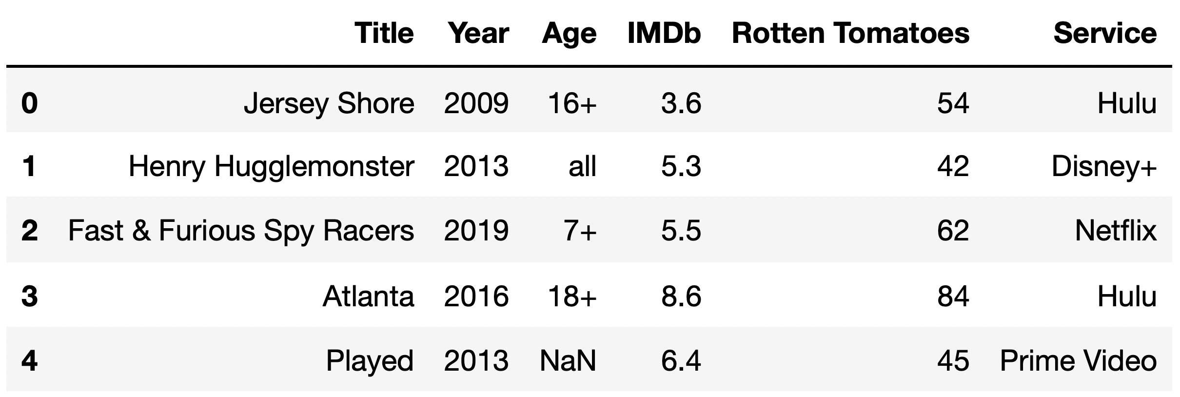
Given no other information other than a TV show’s "Title" and "IMDb" rating, what is the most likely missingness mechanism of the "IMDb" column?
A. Missing by design
B. Not missing at random
C. Missing at random
D. Missing completely at random
Question 🤔 (Answer at dsc80.com/q)
Code: lec08-imdb2
Taken from the Winter 2023 DSC 80 Midterm Exam.
Now, suppose we discover that the median "Rotten Tomatoes" rating among TV shows with a missing "IMDb" rating is a 13, while the median "Rotten Tomatoes" rating among TV shows with a present "IMDb" rating is a 52.
Given this information, what is the most likely missingness mechanism of the "IMDb" column?
A. Missing by design
B. Not missing at random
C. Missing at random
D. Missing completely at random
Question 🤔 (Answer at dsc80.com/q)
Code: lec08-blood
Suppose Sam collects the blood pressures of 30 people in January. Then, in February, he asks a subset of the people to come back for a second reading (which means that there are missing blood pressures for February). What are the missing mechanisms for the blood pressures in February in the following situations?
- Sam uses
np.random.choice()to select 7 individuals from January. - Sam asks the individuals who had hypertension (blood pressure > 140) in January to come back in February.
- Sam asks everyone to come back for a second reading in February, but only records the data for people who had hypertension (blood pressure > 140).
Identifying missingness mechanisms in data
Example: Heights
- Let's load in Galton's dataset containing the heights of adult children and their parents (which you may have seen in DSC 10).
- The dataset does not contain any missing values – we will artifically introduce missing values such that the values are MCAR, for illustration.
heights_path = Path('data') / 'midparent.csv'
heights = pd.read_csv(heights_path).rename(columns={'childHeight': 'child'})[['father', 'mother', 'gender', 'child']]
heights.head()
| father | mother | gender | child | |
|---|---|---|---|---|
| 0 | 78.5 | 67.0 | male | 73.2 |
| 1 | 78.5 | 67.0 | female | 69.2 |
| 2 | 78.5 | 67.0 | female | 69.0 |
| 3 | 78.5 | 67.0 | female | 69.0 |
| 4 | 75.5 | 66.5 | male | 73.5 |
Simulating MCAR data
- We will make
'child'MCAR by taking a random subset ofheightsand setting the corresponding'child'heights tonp.NaN. - This is equivalent to flipping a (biased) coin for each row.
- If heads, we delete the
'child'height.
- If heads, we delete the
- You will not do this in practice!
np.random.seed(42) # So that we get the same results each time (for lecture).
heights_mcar = heights.copy()
idx = heights_mcar.sample(frac=0.3).index
heights_mcar.loc[idx, 'child'] = np.nan
heights_mcar.head(10)
| father | mother | gender | child | |
|---|---|---|---|---|
| 0 | 78.5 | 67.0 | male | 73.2 |
| 1 | 78.5 | 67.0 | female | 69.2 |
| 2 | 78.5 | 67.0 | female | NaN |
| ... | ... | ... | ... | ... |
| 7 | 75.5 | 66.5 | female | NaN |
| 8 | 75.0 | 64.0 | male | 71.0 |
| 9 | 75.0 | 64.0 | female | 68.0 |
10 rows × 4 columns
heights_mcar.isna().mean()
father 0.0 mother 0.0 gender 0.0 child 0.3 dtype: float64
Verifying that child heights are MCAR in heights_mcar
- Each row of
heights_mcarbelongs to one of two groups:- Group 1:
'child'is missing. - Group 2:
'child'is not missing.
- Group 1:
heights_mcar['child_missing'] = heights_mcar['child'].isna()
heights_mcar.head()
| father | mother | gender | child | child_missing | |
|---|---|---|---|---|---|
| 0 | 78.5 | 67.0 | male | 73.2 | False |
| 1 | 78.5 | 67.0 | female | 69.2 | False |
| 2 | 78.5 | 67.0 | female | NaN | True |
| 3 | 78.5 | 67.0 | female | 69.0 | False |
| 4 | 75.5 | 66.5 | male | 73.5 | False |
- We need to look at the distributions of every other column –
'gender','mother', and'father'– separately for these two groups, and check to see if they are similar.
gender_dist = (
heights_mcar
.assign(child_missing=heights_mcar['child'].isna())
.pivot_table(index='gender', columns='child_missing', aggfunc='size')
)
# Added just to make the resulting pivot table easier to read.
gender_dist.columns = ['child_missing = False', 'child_missing = True']
gender_dist = gender_dist / gender_dist.sum()
gender_dist
| child_missing = False | child_missing = True | |
|---|---|---|
| gender | ||
| female | 0.49 | 0.48 |
| male | 0.51 | 0.52 |
gender_dist.plot(kind='barh', title='Gender by Missingness of Child Height (MCAR Example)', barmode='group')
Since 'gender' is categorical, we're looking at two categorical variables here. The two distributions look similar, but to make formal what we mean by similar, we'd need to run a permutation test.
create_kde_plotly(heights_mcar, 'child_missing', True, False, 'father',
"Father's Height by Missingness of Child Height (MCAR Example)")
Since 'father's heights are numerical, we're looking at two numerical variables here. The two distributions look similar, but to make formal what we mean by similar, we'd need to run a permutation test.
create_kde_plotly(heights_mcar, 'child_missing', True, False, 'mother',
"Mother's Height by Missingness of Child Height (MCAR Example)")
Again, 'mother's heights are numerical, we're looking at two numerical variables here. The two distributions look similar, but to make formal what we mean by similar, we'd need to run a permutation test.
Concluding that 'child' is MCAR
We need to run three permutation tests – one for each column in
heights_mcarother than'child'.For every other column, if we fail to reject the null that the distribution of the column when
'child'is missing is the same as the distribution of the column when'child'is not missing, then we can conclude'child'is MCAR.- In such a case, its missingness is not tied to any other columns.
- For instance, children with shorter fathers are not any more likely to have missing heights than children with taller fathers.
Simulating MAR data
Now, we will make 'child' heights MAR by deleting 'child' heights according to a random procedure that depends on other columns.
np.random.seed(42) # So that we get the same results each time (for lecture).
def make_missing(r):
rand = np.random.uniform() # Random real number between 0 and 1.
if r['father'] > 72 and rand < 0.5:
return np.nan
elif r['gender'] == 'female' and rand < 0.3:
return np.nan
else:
return r['child']
heights_mar = heights.copy()
heights_mar['child'] = heights_mar.apply(make_missing, axis=1)
heights_mar['child_missing'] = heights_mar['child'].isna()
heights_mar.head()
| father | mother | gender | child | child_missing | |
|---|---|---|---|---|---|
| 0 | 78.5 | 67.0 | male | NaN | True |
| 1 | 78.5 | 67.0 | female | 69.2 | False |
| 2 | 78.5 | 67.0 | female | 69.0 | False |
| 3 | 78.5 | 67.0 | female | 69.0 | False |
| 4 | 75.5 | 66.5 | male | NaN | True |
Comparing null and non-null 'child' distributions for 'gender', again
This time, the distribution of 'gender' in the two groups is very different.
gender_dist = (
heights_mar
.assign(child_missing=heights_mar['child'].isna())
.pivot_table(index='gender', columns='child_missing', aggfunc='size')
)
# Added just to make the resulting pivot table easier to read.
gender_dist.columns = ['child_missing = False', 'child_missing = True']
gender_dist = gender_dist / gender_dist.sum()
gender_dist
| child_missing = False | child_missing = True | |
|---|---|---|
| gender | ||
| female | 0.4 | 0.88 |
| male | 0.6 | 0.12 |
gender_dist.plot(kind='barh', title='Gender by Missingness of Child Height (MAR Example)', barmode='group')
Comparing null and non-null 'child' distributions for 'father', again
create_kde_plotly(heights_mar, 'child_missing', True, False, 'father',
"Father's Height by Missingness of Child Height (MAR Example)")
- The above two distributions look quite different.
- This is because we artificially created missingness in the dataset in a way that depended on
'father'and'gender'.
- This is because we artificially created missingness in the dataset in a way that depended on
- However, their difference in means is small:
(
heights_mar
.groupby('child_missing')
['father']
.mean()
.diff()
.iloc[-1]
)
np.float64(1.0055466604787853)
- If we ran a permutation test with the difference in means as our test statistic, we would fail to reject the null.
- Using just the difference in means, it is hard to tell these two distributions apart.
The Kolmogorov-Smirnov test statistic
Recap: Permutation tests
- Permutation tests help decide whether two samples look like they were drawn from the same population distribution.
- In a permutation test, we simulate data under the null by shuffling either group labels or numerical features.
- In effect, this randomly assigns individuals to groups.
- If the two distributions are numerical, we've used as our test statistic the difference in group means or medians.
- If the two distributions are categorical, we've used as our test statistic the total variation distance (TVD).
Difference in means
The difference in means works well in some cases. Let's look at one such case.
Below, we artificially generate two numerical datasets.
np.random.seed(42) # So that we get the same results each time (for lecture).
N = 1000 # Number of samples for each distribution.
# Distribution 'A'.
distr1 = pd.Series(np.random.normal(0, 1, size=N // 2))
# Distribution 'B'.
distr2 = pd.Series(np.random.normal(3, 1, size=N // 2))
data = pd.concat([distr1, distr2], axis=1, keys=['A', 'B']).unstack().reset_index().drop('level_1', axis=1)
data = data.rename(columns={'level_0': 'group', 0: 'data'})
meanA, meanB = data.groupby('group')['data'].mean().round(7).tolist()
create_kde_plotly(data, 'group', 'A', 'B', 'data', f'mean of A: {meanA}<br>mean of B: {meanB}')
Different distributions with the same mean
Let's generate two distributions that look very different but have the same mean.
np.random.seed(42) # So that we get the same results each time (for lecture).
N = 1000 # Number of samples for each distribution.
# Distribution 'A'.
a = pd.Series(np.random.normal(0, 1, size=N//2))
b = pd.Series(np.random.normal(4, 1, size=N//2))
distr1 = pd.concat([a,b], ignore_index=True)
# Distribution 'B'.
distr2 = pd.Series(np.random.normal(distr1.mean(), distr1.std(), size=N))
data = pd.concat([distr1, distr2], axis=1, keys=['A', 'B']).unstack().reset_index().drop('level_1', axis=1)
data = data.rename(columns={'level_0': 'group', 0: 'data'})
meanA, meanB = data.groupby('group')['data'].mean().round(7).tolist()
create_kde_plotly(data, 'group', 'A', 'B', 'data', f'mean of A: {meanA}<br>mean of B: {meanB}')
In this case, if we use the difference in means as our test statistic in a permutation test, we will fail to reject the null that the two distributions are different.
n_repetitions = 500
shuffled = data.copy()
diff_means = []
for _ in range(n_repetitions):
# Shuffling the values, while keeping the group labels in place.
shuffled['data'] = np.random.permutation(shuffled['data'])
# Computing and storing the absolute difference in means.
diff_mean = shuffled.groupby('group')['data'].mean().diff().abs().iloc[-1]
diff_means.append(diff_mean)
observed_diff = data.groupby('group')['data'].mean().diff().abs().iloc[-1]
fig = px.histogram(pd.DataFrame(diff_means), x=0, nbins=50, histnorm='probability',
title='Empirical Distribution of the Absolute Difference in Means')
fig.add_vline(x=observed_diff, line_color='red', line_width=1, opacity=1)
fig.add_annotation(text=f'<span style="color:red">Observed Absolute Difference in Means = {round(observed_diff, 2)}</span>',
x=2 * observed_diff, showarrow=False, y=0.07)
# The computed p-value is fairly large.
np.mean(np.array(diff_means) >= observed_diff)
np.float64(0.108)
Telling numerical distributions apart
- The difference in means only works as a test statistic in permutation tests if the two distributions have similar shapes.
- It tests to see if one is a shifted version of the other.
- We need a better test statistic to differentiate between numerical distributions with different shapes.
- In other words, we need a distance metric between numerical.
- The TVD is a distance metric between categorical distributions.
create_kde_plotly(data, 'group', 'A', 'B', 'data', f'mean of A: {meanA}<br>mean of B: {meanB}')
The Kolmogorov-Smirnov test statistic
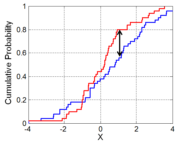
- The K-S test statistic measures the similarity between two distributions.
- It is defined in terms of the cumulative distribution function (CDF) of a given distribution.
- If $f(x)$ is a distribution, then the CDF $F(x)$ is the proportion of values in distribution $f$ that are less than or equal to $x$.
- The K-S statistic is roughly defined as the largest difference between two CDFs.
Aside: Cumulative distribution functions
First, some setup.
fig1 = create_kde_plotly(data, 'group', 'A', 'B', 'data', f'Distributions of A and B')
# Think about what this function is doing!
def create_cdf(group):
return data.loc[data['group'] == group, 'data'].value_counts(normalize=True).sort_index().cumsum()
fig2 = go.Figure()
fig2.add_trace(
go.Scatter(x=create_cdf('A').index, y=create_cdf('A'), name='CDF of A')
)
fig2.add_trace(
go.Scatter(x=create_cdf('B').index, y=create_cdf('B'), name='CDF of B')
)
fig2.update_layout(title='CDFs of A and B')
from plotly.subplots import make_subplots
for i in range(2):
fig2.data[i]['marker']['color'] = fig1.data[i]['marker']['color']
fig2.data[i]['showlegend'] = False
fig = make_subplots(rows=1, cols=2, subplot_titles=['Distributions', 'CDFs'])
fig.add_trace(fig1.data[0], row=1, col=1)
fig.add_trace(fig1.data[1], row=1, col=1)
fig.add_trace(fig2.data[0], row=1, col=2)
fig.add_trace(fig2.data[1], row=1, col=2)
fig.update_layout(width=1000, height=400);
Aside: Cumulative distribution functions
Let's look at the CDFs of our two synthetic distributions.
fig
The K-S statistic in Python
Fortunately, we don't need to calculate the K-S statistic ourselves! Python can do it for us (and you can use this pre-built version in all assignments).
from scipy.stats import ks_2samp
ks_2samp?
Signature: ks_2samp( data1, data2, alternative='two-sided', method='auto', *, axis=0, nan_policy='propagate', keepdims=False, ) Docstring: Performs the two-sample Kolmogorov-Smirnov test for goodness of fit. This test compares the underlying continuous distributions F(x) and G(x) of two independent samples. See Notes for a description of the available null and alternative hypotheses. Parameters ---------- data1, data2 : array_like, 1-Dimensional Two arrays of sample observations assumed to be drawn from a continuous distribution, sample sizes can be different. alternative : {'two-sided', 'less', 'greater'}, optional Defines the null and alternative hypotheses. Default is 'two-sided'. Please see explanations in the Notes below. method : {'auto', 'exact', 'asymp'}, optional Defines the method used for calculating the p-value. The following options are available (default is 'auto'): * 'auto' : use 'exact' for small size arrays, 'asymp' for large * 'exact' : use exact distribution of test statistic * 'asymp' : use asymptotic distribution of test statistic axis : int or None, default: 0 If an int, the axis of the input along which to compute the statistic. The statistic of each axis-slice (e.g. row) of the input will appear in a corresponding element of the output. If ``None``, the input will be raveled before computing the statistic. nan_policy : {'propagate', 'omit', 'raise'} Defines how to handle input NaNs. - ``propagate``: if a NaN is present in the axis slice (e.g. row) along which the statistic is computed, the corresponding entry of the output will be NaN. - ``omit``: NaNs will be omitted when performing the calculation. If insufficient data remains in the axis slice along which the statistic is computed, the corresponding entry of the output will be NaN. - ``raise``: if a NaN is present, a ``ValueError`` will be raised. keepdims : bool, default: False If this is set to True, the axes which are reduced are left in the result as dimensions with size one. With this option, the result will broadcast correctly against the input array. Returns ------- res: KstestResult An object containing attributes: statistic : float KS test statistic. pvalue : float One-tailed or two-tailed p-value. statistic_location : float Value from `data1` or `data2` corresponding with the KS statistic; i.e., the distance between the empirical distribution functions is measured at this observation. statistic_sign : int +1 if the empirical distribution function of `data1` exceeds the empirical distribution function of `data2` at `statistic_location`, otherwise -1. See Also -------- :func:`kstest`, :func:`ks_1samp`, :func:`epps_singleton_2samp`, :func:`anderson_ksamp` .. Notes ----- There are three options for the null and corresponding alternative hypothesis that can be selected using the `alternative` parameter. - `less`: The null hypothesis is that F(x) >= G(x) for all x; the alternative is that F(x) < G(x) for at least one x. The statistic is the magnitude of the minimum (most negative) difference between the empirical distribution functions of the samples. - `greater`: The null hypothesis is that F(x) <= G(x) for all x; the alternative is that F(x) > G(x) for at least one x. The statistic is the maximum (most positive) difference between the empirical distribution functions of the samples. - `two-sided`: The null hypothesis is that the two distributions are identical, F(x)=G(x) for all x; the alternative is that they are not identical. The statistic is the maximum absolute difference between the empirical distribution functions of the samples. Note that the alternative hypotheses describe the *CDFs* of the underlying distributions, not the observed values of the data. For example, suppose x1 ~ F and x2 ~ G. If F(x) > G(x) for all x, the values in x1 tend to be less than those in x2. If the KS statistic is large, then the p-value will be small, and this may be taken as evidence against the null hypothesis in favor of the alternative. If ``method='exact'``, `ks_2samp` attempts to compute an exact p-value, that is, the probability under the null hypothesis of obtaining a test statistic value as extreme as the value computed from the data. If ``method='asymp'``, the asymptotic Kolmogorov-Smirnov distribution is used to compute an approximate p-value. If ``method='auto'``, an exact p-value computation is attempted if both sample sizes are less than 10000; otherwise, the asymptotic method is used. In any case, if an exact p-value calculation is attempted and fails, a warning will be emitted, and the asymptotic p-value will be returned. The 'two-sided' 'exact' computation computes the complementary probability and then subtracts from 1. As such, the minimum probability it can return is about 1e-16. While the algorithm itself is exact, numerical errors may accumulate for large sample sizes. It is most suited to situations in which one of the sample sizes is only a few thousand. We generally follow Hodges' treatment of Drion/Gnedenko/Korolyuk [1]_. Beginning in SciPy 1.9, ``np.matrix`` inputs (not recommended for new code) are converted to ``np.ndarray`` before the calculation is performed. In this case, the output will be a scalar or ``np.ndarray`` of appropriate shape rather than a 2D ``np.matrix``. Similarly, while masked elements of masked arrays are ignored, the output will be a scalar or ``np.ndarray`` rather than a masked array with ``mask=False``. References ---------- .. [1] Hodges, J.L. Jr., "The Significance Probability of the Smirnov Two-Sample Test," Arkiv fiur Matematik, 3, No. 43 (1958), 469-486. Examples -------- Suppose we wish to test the null hypothesis that two samples were drawn from the same distribution. We choose a confidence level of 95%; that is, we will reject the null hypothesis in favor of the alternative if the p-value is less than 0.05. If the first sample were drawn from a uniform distribution and the second were drawn from the standard normal, we would expect the null hypothesis to be rejected. >>> import numpy as np >>> from scipy import stats >>> rng = np.random.default_rng() >>> sample1 = stats.uniform.rvs(size=100, random_state=rng) >>> sample2 = stats.norm.rvs(size=110, random_state=rng) >>> stats.ks_2samp(sample1, sample2) KstestResult(statistic=0.5454545454545454, pvalue=7.37417839555191e-15, statistic_location=-0.014071496412861274, statistic_sign=-1) Indeed, the p-value is lower than our threshold of 0.05, so we reject the null hypothesis in favor of the default "two-sided" alternative: the data were *not* drawn from the same distribution. When both samples are drawn from the same distribution, we expect the data to be consistent with the null hypothesis most of the time. >>> sample1 = stats.norm.rvs(size=105, random_state=rng) >>> sample2 = stats.norm.rvs(size=95, random_state=rng) >>> stats.ks_2samp(sample1, sample2) KstestResult(statistic=0.10927318295739348, pvalue=0.5438289009927495, statistic_location=-0.1670157701848795, statistic_sign=-1) As expected, the p-value of 0.54 is not below our threshold of 0.05, so we cannot reject the null hypothesis. Suppose, however, that the first sample were drawn from a normal distribution shifted toward greater values. In this case, the cumulative density function (CDF) of the underlying distribution tends to be *less* than the CDF underlying the second sample. Therefore, we would expect the null hypothesis to be rejected with ``alternative='less'``: >>> sample1 = stats.norm.rvs(size=105, loc=0.5, random_state=rng) >>> stats.ks_2samp(sample1, sample2, alternative='less') KstestResult(statistic=0.4055137844611529, pvalue=3.5474563068855554e-08, statistic_location=-0.13249370614972575, statistic_sign=-1) and indeed, with p-value smaller than our threshold, we reject the null hypothesis in favor of the alternative. File: ~/miniforge3/envs/dsc80/lib/python3.11/site-packages/scipy/stats/_stats_py.py Type: function
observed_ks = ks_2samp(data.loc[data['group'] == 'A', 'data'], data.loc[data['group'] == 'B', 'data']).statistic
observed_ks
np.float64(0.14)
We don't know if this number is big or small. We need to run a permutation test!
n_repetitions = 500
shuffled = data.copy()
ks_stats = []
for _ in range(n_repetitions):
# Shuffling the data.
shuffled['data'] = np.random.permutation(shuffled['data'])
# Computing and storing the K-S statistic.
groups = shuffled.groupby('group')['data']
ks_stat = ks_2samp(groups.get_group('A'), groups.get_group('B')).statistic
ks_stats.append(ks_stat)
ks_stats[:10]
[np.float64(0.027), np.float64(0.07), np.float64(0.035), np.float64(0.021), np.float64(0.055), np.float64(0.029), np.float64(0.033), np.float64(0.026), np.float64(0.073), np.float64(0.039)]
fig = px.histogram(pd.DataFrame(ks_stats), x=0, nbins=50, histnorm='probability',
title='Empirical Distribution of the K-S Statistic')
fig.add_vline(x=observed_ks, line_color='red', line_width=1, opacity=1)
fig.add_annotation(text=f'<span style="color:red">Observed KS = {round(observed_ks, 2)}</span>',
x=0.8 * observed_ks, showarrow=False, y=0.16)
fig.update_layout(xaxis_range=[0, 0.2])
fig.update_layout(yaxis_range=[0, 0.2])
np.mean(np.array(ks_stats) >= observed_ks)
np.float64(0.0)
We were able to differentiate between the two distributions using the K-S test statistic!
ks_2samp
scipy.stats.ks_2sampactually returns both the statistic and a p-value.- The p-value is calculated using the permutation test we just performed!
ks_2samp(data.loc[data['group'] == 'A', 'data'], data.loc[data['group'] == 'B', 'data'])
KstestResult(statistic=np.float64(0.14), pvalue=np.float64(5.822752148022591e-09), statistic_location=np.float64(0.9755451271223592), statistic_sign=np.int8(1))
Difference in means vs. K-S statistic
- The K-S statistic measures the difference between two numerical distributions.
- It does not quantify if one is larger than the other on average, so there are times we still need to use the difference in means.
- Strategy: Always plot the two distributions you are comparing.
- If the distributions have similar shapes but are centered in different places, use the difference in means (or absolute difference in means).
- If your alternative hypothesis involves a "direction" (i.e. smoking weights were are on average than non-smoking weights), use the difference in means.
- If the distributions have different shapes but roughly the same center, and your alternative hypothesis is simply that the two distributions are different, use the K-S statistic.
Back to our Example: Missingness of 'child' heights on 'father''s heights (MAR)
heights_mar['child_missing'] = heights_mar['child'].isna()
create_kde_plotly(heights_mar[['child_missing', 'father']], 'child_missing', True, False, 'father',
"Father's Height by Missingness of Child Height (MAR example)")
The above picture shows us that missing
'child'heights tend to come from taller'father's heights.To determine whether the two distributions are significantly different, we must use a permutation test. This time, the difference in means is not a good choice, since the centers are similar but the shapes are different.
Performing the test
heights_mar
| father | mother | gender | child | child_missing | |
|---|---|---|---|---|---|
| 0 | 78.5 | 67.0 | male | NaN | True |
| 1 | 78.5 | 67.0 | female | 69.2 | False |
| 2 | 78.5 | 67.0 | female | 69.0 | False |
| ... | ... | ... | ... | ... | ... |
| 931 | 62.0 | 66.0 | female | 61.0 | False |
| 932 | 62.5 | 63.0 | male | 66.5 | False |
| 933 | 62.5 | 63.0 | female | 57.0 | False |
934 rows × 5 columns
ks_2samp(heights_mar.query('child_missing')['father'], heights_mar.query('not child_missing')['father'])
KstestResult(statistic=np.float64(0.20676025834396874), pvalue=np.float64(1.1424922868036869e-05), statistic_location=np.float64(72.0), statistic_sign=np.int8(-1))
The p-value is very small, so we conclude that the child height is MAR, conditional on the father's height.
Handling missing values
What do we do with missing data?
- Suppose we are interested in a dataset $Y$.
- We get to observe $Y_{obs}$, while the rest of the dataset, $Y_{mis}$, is missing.
- Issue: $Y_{obs}$ may look quite different than $Y$.
- The mean and other measures of central tendency may be different.
- The variance may be different.
- The correlations between variables may be different.
Solution 1: Dropping missing values
- If the data are MCAR (missing completely at random), then dropping the missing values entirely doesn't significantly change the data.
- For instance, the mean of the dataset post-dropping is an unbiased estimate of the true mean.
- This is because MCAR data is a random sample of the full dataset.
- From DSC 10, we know that random samples tend to resemble the larger populations they are drawn from.
- If the data are not MCAR, then dropping the missing values will introduce bias.
- MCAR is rare!
- For instance, suppose we asked people "How much do you give to charity?" People who give little are less likely to respond, so the average response is biased high.
Listwise deletion
- Listwise deletion is the act of dropping entire rows that contain missing values.
- Issue: This can delete perfectly good data in other columns for a given row.
- Improvement: Drop missing data only when working with the column that contains missing data.
To illustrate, let's generate two datasets with missing 'child' heights – one in which the heights are MCAR, and one in which they are MAR dependent on 'gender' only.
In practice, you'll have to run permutation tests to determine the likely missingness mechanism first!
np.random.seed(42) # So that we get the same results each time (for lecture).
heights_mcar = make_mcar(heights, 'child', pct=0.5)
heights_mar = make_mar_on_cat(heights, 'child', 'gender', pct=0.5)
Listwise deletion
Below, we compute the means and standard deviations of the 'child' column in all three datasets. Remember, .mean() and .std() ignore missing values.
multiple_describe({
'Original': heights,
'MCAR': heights_mcar,
'MAR': heights_mar
})
| Mean | Standard Deviation | |
|---|---|---|
| Dataset | ||
| Original | 66.75 | 3.58 |
| MCAR | 66.64 | 3.56 |
| MAR | 68.52 | 3.12 |
Observations:
The
'child'mean (and SD) in the MCAR dataset is very close to the true'child'mean (and SD).The
'child'mean in the MAR dataset is biased high.
Solution 2: Imputation
Imputation is the act of filling in missing data with plausable values. Ideally, imputation:
- is quick and easy to do.
- shouldn't introduce bias into the dataset.
These are hard to do at the same time!
Kinds of imputation
There are three main types of imputation, two of which we will focus on today:
- Imputation with a single value: mean, median, mode.
- Imputation with a single value, using a model: regression, kNN.
- Probabilistic imputation by drawing from a distribution.
Each has upsides and downsides, and each works differently with different types of missingness.
Mean imputation
Mean imputation
- Mean imputation is the act of filling in missing values in a column with the mean of the observed values in that column.
- This strategy:
- 👍 Preserves the mean of the observed data, for all types of missingness.
- 👎 Decreases the variance of the data, for all types of missingness.
- 👎 Creates a biased estimate of the true mean when the data are not MCAR.
Example: Mean imputation in the MCAR heights dataset
Let's look at two distributions:
- The distribution of the
'child'column inheights, where we have all the data. - The distribution of the
'child'column inheights_mcar, where some values are MCAR.
# Look in util.py to see how multiple_kdes is defined.
multiple_kdes({'Original': heights, 'MCAR, Unfilled': heights_mcar})
- Since the
'child'heights are MCAR, the orange distribution, in which some values are missing, has roughly the same shape as the turquoise distribution, which has no missing values.
Mean imputation of MCAR data
Let's fill in missing values in heights_mcar['child'] with the mean of the observed 'child' heights in heights_mcar['child'].
heights_mcar['child'].head()
heights_mcar_mfilled = heights_mcar.fillna(heights_mcar['child'].mean())
heights_mcar_mfilled['child'].head()
df_map = {'Original': heights, 'MCAR, Unfilled': heights_mcar, 'MCAR, Mean Imputed': heights_mcar_mfilled}
multiple_describe(df_map)
Observations:
The mean of the imputed dataset is the same as the mean of the subset of heights that aren't missing (which is close to the true mean).
The standard deviation of the imputed dataset smaller than that of the other two datasets. Why?
Mean imputation of MCAR data
Let's visualize all three distributions: the original, the MCAR heights with missing values, and the mean-imputed MCAR heights.
multiple_kdes(df_map)
Takeaway: When data are MCAR and you impute with the mean:
- The mean of the imputed dataset is an unbiased estimator of the true mean.
- The variance of the imputed dataset is smaller than the variance of the full dataset.
- Mean imputation tricks you into thinking your data are more reliable than they are!
Example: Mean imputation in the MAR heights dataset
When data are MAR, mean imputation leads to biased estimates of the mean across groups.
The bias may be different in different groups.
- For example: If the missingness depends on gender, then different genders will have differently-biased means.
- The overall mean will be biased towards one group.
Again, let's look at two distributions:
- The distribution of the
'child'column inheights, where we have all the data. - The distribution of the
'child'column inheights_mar, where some values are MAR.
- The distribution of the
multiple_kdes({'Original': heights, 'MAR, Unfilled': heights_mar})
The distributions are not very similar!
Remember that in reality, you won't get to see the turquoise distribution, which has no missing values – instead, you'll try to recreate it, using your sample with missing values.
Mean imputation of MAR data
Let's fill in missing values in heights_mar['child'] with the mean of the observed 'child' heights in heights_mar['child'] and see what happens.
heights_mar['child'].head()
heights_mar_mfilled = heights_mar.fillna(heights_mar['child'].mean())
heights_mar_mfilled['child'].head()
df_map = {'Original': heights, 'MAR, Unfilled': heights_mar, 'MAR, Mean Imputed': heights_mar_mfilled}
multiple_describe(df_map)
Note that the latter two means are biased high.
Mean imputation of MAR data
Let's visualize all three distributions: the original, the MAR heights with missing values, and the mean-imputed MAR heights.
multiple_kdes(df_map)
Since the sample with MAR values was already biased high, mean imputation kept the sample biased – it did not bring the data closer to the data generating process.
With our single mean imputation strategy, the resulting female mean height is biased quite high.
pd.concat([
heights.groupby('gender')['child'].mean().rename('Original'),
heights_mar.groupby('gender')['child'].mean().rename('MAR, Unfilled'),
heights_mar_mfilled.groupby('gender')['child'].mean().rename('MAR, Mean Imputed')
], axis=1).T
Within-group (conditional) mean imputation
- Improvement: Since MAR data are MCAR within each group, we can perform group-wise mean imputation.
- In our case, since the missingness of
'child'is dependent on'gender', we can impute separately for each'gender'. - For instance, if there is a missing
'child'height for a'female'child, impute their height with the mean observed'female'height.
- In our case, since the missingness of
With this technique, the overall mean remains unbiased, as do the within-group means.
Like with "single" mean imputation, the variance of the dataset is reduced.
transform returns!
- In MAR data, imputation by the overall mean gives a biased estimate of the mean of each group.
- To obtain an unbiased estimate of the mean within each group, impute using the mean within each group.
- To perform an operation separately to each gender, we
groupby('gender')and use thetransformmethod.
def mean_impute(s):
return s.fillna(s.mean())
heights_mar_cond = heights_mar.groupby('gender')['child'].transform(mean_impute).to_frame()
heights_mar_cond['child'].head()
df_map['MAR, Conditional Mean Imputed'] = heights_mar_cond
multiple_kdes(df_map)
The pink distribution does a slightly better job of approximating the turquoise distribution than the purple distribution, but not by much.
Conclusion: Imputation with single values
Imputing missing data in a column with the mean of the column:
- faithfully reproduces the mean of the observed dataset,
- reduces the variance, and
- biases relationships between the column and other columns if the data are not MCAR.
The same is true with other statistics (e.g. median and mode).
Probabilistic imputation
Imputing missing values using distributions
- So far, each missing value in a column has been filled in with a constant value.
- This creates "spikes" in the imputed distributions.
- Idea: We can probabilistically impute missing data from a distribution.
- We can fill in missing data by drawing from the distribution of the non-missing data.
- There are 5 missing values? Pick 5 values from the data that aren't missing.
- How? Using
np.random.choiceor.sample.
- If the data are MCAR, then sample from the entire column of present values. If the data are MAR on some categorical column, then sample from the present values separately for each category.
Example: Probabilistic imputation in the MAR heights dataset
Let's use transform to call prob_impute separately on each 'gender'.
def prob_impute(s):
s = s.copy()
# Step 1: Find the number of missing child heights for that gender.
num_null = s.isna().sum()
# Step 2: Sample num_null observed child heights for that gender.
fill_values = np.random.choice(s.dropna(), num_null)
# Step 3: Fill in missing values and return ser.
s[s.isna()] = fill_values
return s
heights_mar_pfilled = heights_mar.copy()
heights_mar_pfilled['child'] = (
heights_mar
.groupby('gender')
['child']
.transform(prob_impute)
)
heights_mar_pfilled['child'].head()
df_map['MAR, Conditionally Probabilistically Imputed'] = heights_mar_pfilled
multiple_kdes(df_map)
The green distribution (conditional probabilistic imputation) does the best job of approximating the turqoise distribution (the full dataset with no missing values)!
Remember that the graph above is interactive – you can hide/show lines by clicking them in the legend.
Observations
With this technique, the missing values were filled in with observed values in the dataset.
If a value was never observed in the dataset, it will never be used to fill in a missing value.
- For instance, if the observed heights were 68, 69, and 69.5 inches, we will never fill a missing value with 68.5 inches even though it's a perfectly reasonable height.
Solution? Create a histogram (with
np.histogram) to bin the data, then sample from the histogram.- See Lab 5, Question 6.
Randomness
Unlike mean imputation, probabilistic imputation is random – each time you run the cell in which imputation is performed, the results could be different.
If we're interested in estimating some population parameter given our (incomplete) sample, it's best not to rely on just a single random imputation.
Multiple imputation: Generate multiple imputed datasets and aggregate the results!
- Similar to bootstrapping.
Question 🤔 (Answer at dsc80.com/q)
Code: lec08-service
Taken from the Winter 2023 DSC 80 Midterm Exam.
To determine whether the missingness of "IMDb" depends on "Service", we produce the following plot.
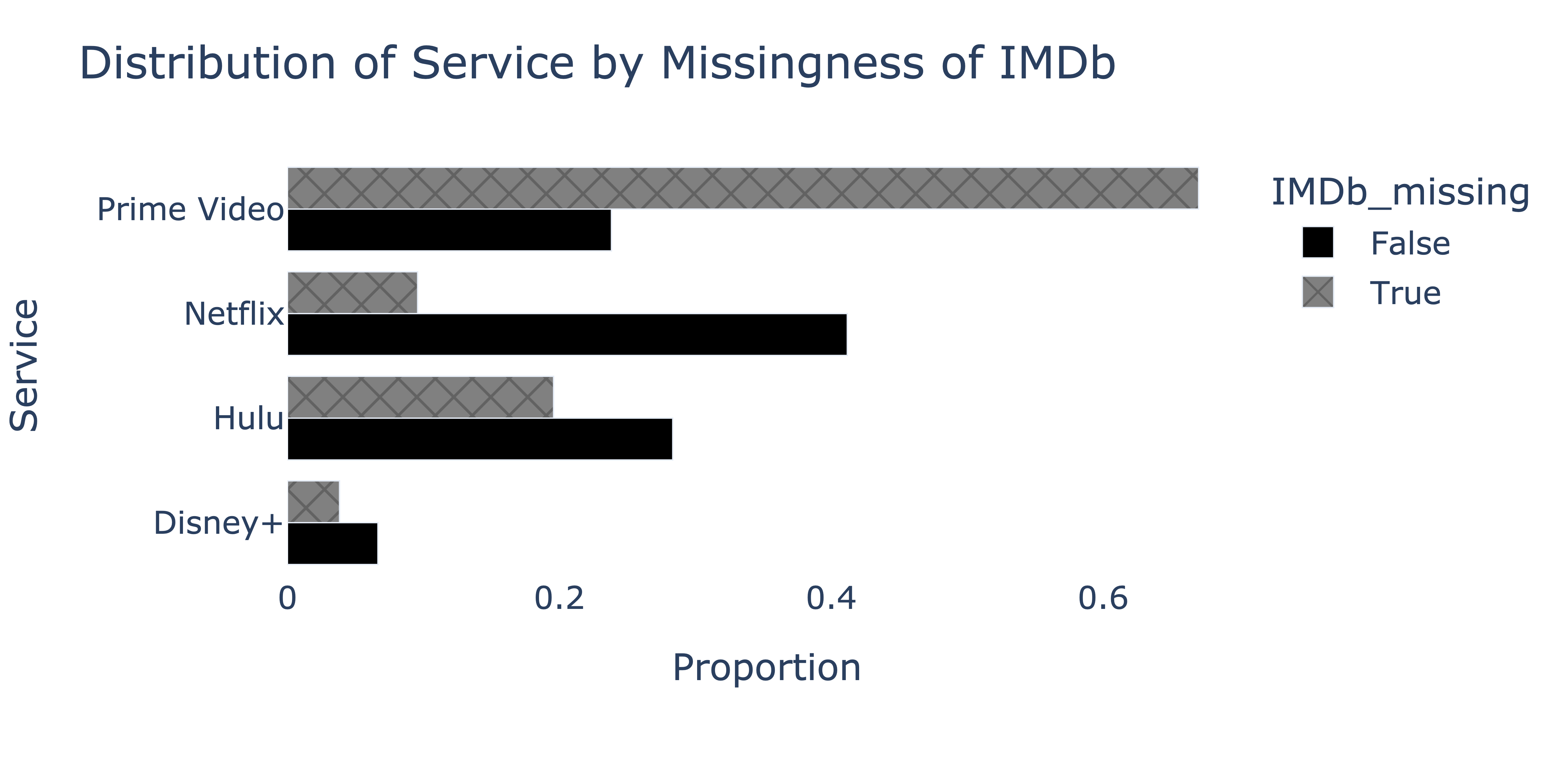
We’d like to fill in missing "IMDb" values in the fastest, most efficient way possible, such that the mean of the imputed "IMDb" column is as close to the true mean of the "IMDb" column in nature as possible. Which imputation technique should we use?
A. Unconditional mean imputation
B. Mean imputation, conditional on "Service"
C. Unconditional probabilistic imputation
D. Probabilistic imputation, conditional on "Service"
Summary, next time
Summary of imputation techniques
- Listwise deletion.
- Mean imputation.
- Group-wise (conditional) mean imputation.
- Probabilistic imputation.
- Multiple imputation.
Summary: Listwise deletion
- Procedure:
df = df.dropna(). - If data are MCAR, listwise deletion doesn't change most summary statistics (mean, median, SD) of the data.
Summary: Mean imputation
- Procedure:
df[col] = df[col].fillna(df[col].mean()). - If data are MCAR, the resulting mean is an unbiased estimate of the true mean, but the variance is too low.
- Analogue for categorical data: imputation with the mode.
Summary: Conditional mean imputation
- Procedure: for a column
c1, conditional on a second categorical columnc2:
means = df.groupby('c2').mean().to_dict()
imputed = df['c1'].apply(lambda x: means[x] if np.isnan(x) else x)
- If data are MAR, the resulting mean is an unbiased estimate of the true mean, but the variance is too low.
- This increases correlations between the columns.
- If the column with missing values were dependent on more than one column, we can use linear regression to predict the missing value.
Summary: Probabilistic imputation
- Procedure: draw from the distribution of observed data to fill in missing values.
- If data are MCAR, the resulting mean and variance are unbiased estimates of the true mean and variance.
- Extending to the MAR case: draw from conditional empirical distributions.
- If data are conditional on a single categorical column
c2, apply the MCAR procedure to the groups ofdf.groupby(c2).
- If data are conditional on a single categorical column
Summary: Multiple imputation
- Procedure:
- Apply probabilistic imputation multiple times, resulting in $m$ imputed datasets.
- Compute statistics separately on the $m$ imputed datasets (e.g. compute the mean or correlation coefficient).
- Plot the distribution of these statistics and create confidence intervals.
- If a column is missing conditional on multiple columns, your "multiple imputations" should include probabilistic imputations for each!
Next time
- Introduction to HTTP.
- Making requests.
- Midterm review
Question 🤔 (Answer at dsc80.com/q)
Code: mt
Take a look at past midterm exams here and submit a question to review next Tuesday.