# You'll start seeing this cell in most lectures.
# It exists to hide all of the import statements and other setup
# code we need in lecture notebooks.

from dsc80_utils import *

Lecture 2 – DataFrame Fundamentals

DSC 80, Spring 2025

Announcements 📣

• Lab 1 is released, and is due Wednesday, April 9 at 11:59pm.
  • See the Tech Support page for instructions on how to set up your environment and work on assignments.
  • Please try to set up your computer ASAP so that you have enough time to debug your environment.
• Project 1 will be released by Friday.
• Please fill out the Welcome Survey ASAP.
• Lecture recordings are available here, and are linked on the course website.

Agenda

• numpy arrays.
• From babypandas to pandas.
  • Deep dive into DataFrames.
• Accessing subsets of rows and columns in DataFrames.
  • .loc and .iloc.
  • Querying (i.e. filtering).
• Adding and modifying columns.
• pandas and numpy.

We can't cover every single detail! The pandas documentation will be your friend.

Question 🤔 (Answer using `lec02-dog`)

dogs = pd.read_csv('data/dogs43.csv')
dogs.head(2)

	breed	kind	lifetime_cost	longevity	size	weight	height
0	Brittany	sporting	22589.0	12.92	medium	35.0	19.0
1	Cairn Terrier	terrier	21992.0	13.84	small	14.0	10.0

What does this code do?

whoa = np.random.choice([True, False], size=len(dogs))
(dogs[whoa]
 .groupby('size')
 .max()
 .get('longevity')
)

size
large     11.92
medium    12.92
small     16.50
Name: longevity, dtype: float64

numpy arrays

numpy overview

• numpy stands for "numerical Python". It is a commonly-used Python module that enables fast computation involving arrays and matrices.
• numpy's main object is the array. In numpy, arrays are:
  • Homogenous – all values are of the same type.
  • (Potentially) multi-dimensional.
• Computation in numpy is fast because:
  • Much of it is implemented in C.
  • numpy arrays are stored more efficiently in memory than, say, Python lists.
• This site provides a good overview of numpy arrays.

We used numpy in DSC 10 to work with sequences of data:

arr = np.arange(10)
arr

array([0, 1, 2, 3, 4, 5, 6, 7, 8, 9])

# The shape (10,) means that the array only has a single dimension,
# of size 10.
arr.shape

(10,)

2 ** arr

array([  1,   2,   4,   8,  16,  32,  64, 128, 256, 512])

Arrays come equipped with several handy methods; some examples are below, but you can read about them all here.

(2 ** arr).sum()

np.int64(1023)

(2 ** arr).mean()

np.float64(102.3)

(2 ** arr).max()

np.int64(512)

(2 ** arr).argmax()

np.int64(9)

⚠️ The dangers of for-loops

• for-loops are slow when processing large datasets. You will rarely write for-loops in DSC 80 (except for Lab 1 and Project 1), and may be penalized on assignments for using them when unnecessary!
• One of the biggest benefits of numpy is that it supports vectorized operations.
  • If a and b are two arrays of the same length, then a + b is a new array of the same length containing the element-wise sum of a and b.
• To illustrate how much faster numpy arithmetic is than using a for-loop, let's compute the squares of the numbers between 0 and 1,000,000:
  • Using a for-loop.
  • Using vectorized arithmetic, through numpy.

%%timeit
squares = []
for i in range(1_000_000):
    squares.append(i * i)

25.8 ms ± 388 μs per loop (mean ± std. dev. of 7 runs, 10 loops each)

In vanilla Python, this takes about 0.04 seconds per loop.

%%timeit
squares = np.arange(1_000_000) ** 2

1.05 ms ± 43.7 μs per loop (mean ± std. dev. of 7 runs, 1,000 loops each)

In numpy, this only takes about 0.001 seconds per loop, more than 40x faster! Note that under the hood, numpy is also using a for-loop, but it's a for-loop implemented in C, which is much faster than Python.

Multi-dimensional arrays

While we didn't see these very often in DSC 10, multi-dimensional lists/arrays may have since come up in DSC 20, 30, or 40A (especially in the context of linear algebra).

We'll spend a bit of time talking about 2D (and 3D) arrays here, since in some ways, they behave similarly to DataFrames.

Below, we create a 2D array from scratch.

nums = np.array([
    [5, 1, 9, 7],
    [9, 8, 2, 3],
    [2, 5, 0, 4]
])

nums

array([[5, 1, 9, 7],
       [9, 8, 2, 3],
       [2, 5, 0, 4]])

# nums has 3 rows and 4 columns.
nums.shape

(3, 4)

We can also create 2D arrays by reshaping other arrays.

# Here, we're asking to reshape np.arange(1, 7)
# so that it has 2 rows and 3 columns.
a = np.arange(1, 7).reshape((2, 3))
a

array([[1, 2, 3],
       [4, 5, 6]])

Operations along axes

In 2D arrays (and DataFrames), axis 0 refers to the rows (up and down) and axis 1 refers to the columns (left and right).

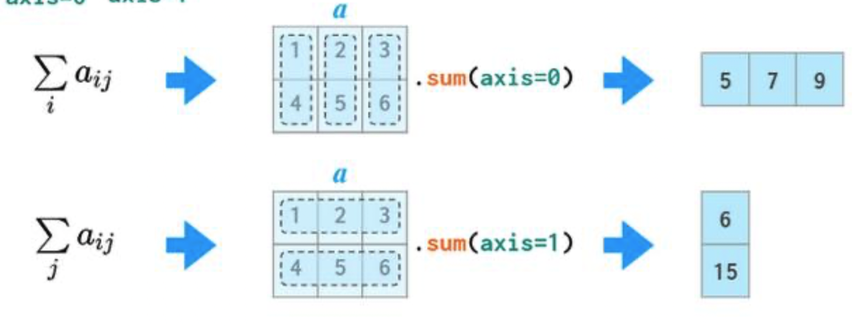
a

array([[1, 2, 3],
       [4, 5, 6]])

If we specify axis=0, a.sum will "compress" along axis 0.

a.sum(axis=0)

array([5, 7, 9])

If we specify axis=1, a.sum will "compress" along axis 1.

a.sum(axis=1)

array([ 6, 15])

Selecting rows and columns from 2D arrays

You can use [square brackets] to slice rows and columns out of an array, using the same slicing conventions you saw in DSC 20.

a

array([[1, 2, 3],
       [4, 5, 6]])

# Accesses row 0 and all columns.
a[0, :]

array([1, 2, 3])

# Same as the above.
a[0]

array([1, 2, 3])

# Accesses all rows and column 1.
a[:, 1]

array([2, 5])

# Accesses row 0 and columns 1 and onwards.
a[0, 1:]

array([2, 3])

Question 🤔 (Answer at `lec02-grid`)

Try and predict the value of grid[-1, 1:].sum() without running the code below.

See if ChatGPT can do it.

s = (5, 3)
grid = np.ones(s) * 2 * np.arange(1, 16).reshape(s)
# grid[-1, 1:].sum()

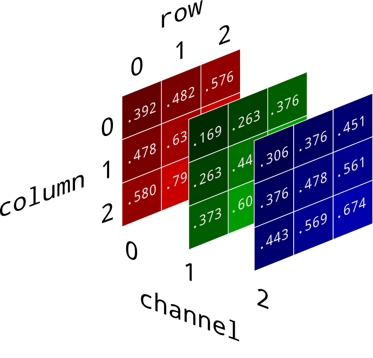
Example: Image processing

numpy arrays are homogenous and potentially multi-dimensional.

It turns out that images can be represented as 3D numpy arrays. The color of each pixel can be described with three numbers under the RGB model – a red value, green value, and blue value. Each of these can vary from 0 to 1.

(image source)

from PIL import Image
img_path = Path('imgs') / 'bentley.jpg'
img = np.asarray(Image.open(img_path)) / 255

img

array([[[0.4 , 0.33, 0.24],
        [0.42, 0.35, 0.25],
        [0.43, 0.36, 0.26],
        ...,
        [0.5 , 0.44, 0.36],
        [0.51, 0.44, 0.36],
        [0.51, 0.44, 0.36]],

       [[0.39, 0.33, 0.23],
        [0.42, 0.36, 0.26],
        [0.44, 0.37, 0.27],
        ...,
        [0.51, 0.44, 0.36],
        [0.52, 0.45, 0.37],
        [0.52, 0.45, 0.38]],

       [[0.38, 0.31, 0.21],
        [0.41, 0.35, 0.24],
        [0.44, 0.37, 0.27],
        ...,
        [0.52, 0.45, 0.38],
        [0.53, 0.46, 0.39],
        [0.53, 0.47, 0.4 ]],

       ...,

       [[0.71, 0.64, 0.55],
        [0.71, 0.65, 0.55],
        [0.68, 0.62, 0.52],
        ...,
        [0.58, 0.49, 0.41],
        [0.56, 0.47, 0.39],
        [0.56, 0.47, 0.39]],

       [[0.5 , 0.44, 0.34],
        [0.42, 0.37, 0.26],
        [0.44, 0.38, 0.28],
        ...,
        [0.4 , 0.33, 0.25],
        [0.55, 0.48, 0.4 ],
        [0.58, 0.5 , 0.42]],

       [[0.38, 0.33, 0.22],
        [0.49, 0.44, 0.33],
        [0.56, 0.51, 0.4 ],
        ...,
        [0.15, 0.08, 0.  ],
        [0.28, 0.21, 0.13],
        [0.42, 0.35, 0.27]]])

img.shape

(200, 263, 3)

plt.imshow(img)
plt.axis('off');

Applying a greyscale filter

One way to convert an image to greyscale is to average its red, green, and blue values.

mean_2d = img.mean(axis=2)
mean_2d

array([[0.32, 0.34, 0.35, ..., 0.43, 0.44, 0.44],
       [0.31, 0.35, 0.36, ..., 0.44, 0.45, 0.45],
       [0.3 , 0.33, 0.36, ..., 0.45, 0.46, 0.47],
       ...,
       [0.64, 0.64, 0.6 , ..., 0.49, 0.47, 0.47],
       [0.43, 0.35, 0.37, ..., 0.32, 0.48, 0.5 ],
       [0.31, 0.42, 0.49, ..., 0.07, 0.21, 0.34]])

This is just a single red channel!

plt.imshow(mean_2d)
plt.axis('off');

We need to repeat mean_2d three times along axis 2, to use the same values for the red, green, and blue channels. np.repeat will help us here.

# np.newaxis is an alias for None.
# It helps us introduce an additional axis.
np.arange(5)[:, np.newaxis]

array([[0],
       [1],
       [2],
       [3],
       [4]])

np.repeat(np.arange(5)[:, np.newaxis], 3, axis=1)

array([[0, 0, 0],
       [1, 1, 1],
       [2, 2, 2],
       [3, 3, 3],
       [4, 4, 4]])

mean_3d = np.repeat(mean_2d[:, :, np.newaxis], 3, axis=2)

plt.imshow(mean_3d)
plt.axis('off');

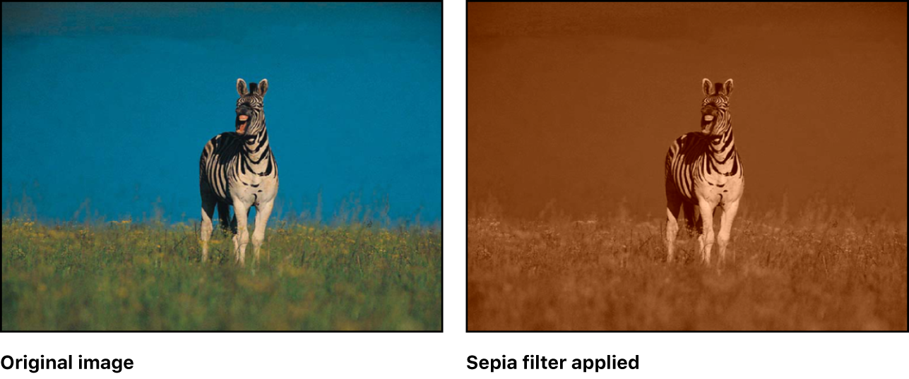
Applying a sepia filter

Let's sepia-fy Junior!

(Image credits)

From here, we can apply this conversion to each pixel.

$$\begin{align*} R_{\text{sepia}} &= 0.393R + 0.769G + 0.189B \\ G_{\text{sepia}} &= 0.349R + 0.686G + 0.168B \\ B_{\text{sepia}} &= 0.272R + 0.534G + 0.131B\end{align*}$$

sepia_filter = np.array([
    [0.393, 0.769, 0.189],
    [0.349, 0.686, 0.168],
    [0.272, 0.534, 0.131]
])

# Multiplies each pixel by the sepia_filter matrix.
# Then, clips each RGB value to be between 0 and 1.
filtered = (img @ sepia_filter.T).clip(0, 1)
filtered

array([[[0.46, 0.41, 0.32],
        [0.48, 0.43, 0.33],
        [0.5 , 0.44, 0.35],
        ...,
        [0.6 , 0.53, 0.42],
        [0.6 , 0.54, 0.42],
        [0.61, 0.54, 0.42]],

       [[0.45, 0.4 , 0.31],
        [0.49, 0.43, 0.34],
        [0.5 , 0.45, 0.35],
        ...,
        [0.61, 0.54, 0.42],
        [0.62, 0.55, 0.43],
        [0.63, 0.56, 0.43]],

       [[0.43, 0.38, 0.3 ],
        [0.47, 0.42, 0.33],
        [0.51, 0.45, 0.35],
        ...,
        [0.63, 0.56, 0.44],
        [0.64, 0.57, 0.44],
        [0.64, 0.57, 0.45]],

       ...,

       [[0.88, 0.78, 0.61],
        [0.89, 0.79, 0.61],
        [0.84, 0.75, 0.58],
        ...,
        [0.68, 0.61, 0.47],
        [0.65, 0.58, 0.45],
        [0.65, 0.58, 0.45]],

       [[0.6 , 0.53, 0.42],
        [0.5 , 0.44, 0.35],
        [0.52, 0.46, 0.36],
        ...,
        [0.45, 0.4 , 0.31],
        [0.66, 0.59, 0.46],
        [0.69, 0.62, 0.48]],

       [[0.45, 0.4 , 0.31],
        [0.59, 0.53, 0.41],
        [0.69, 0.61, 0.48],
        ...,
        [0.12, 0.1 , 0.08],
        [0.3 , 0.26, 0.21],
        [0.48, 0.43, 0.33]]])

plt.imshow(filtered)
plt.axis('off');

Key takeaway: avoid for-loops whenever possible!

You can do a lot without for-loops, both in numpy and in pandas.

From babypandas to pandas 🐼

babypandas

In DSC 10, you used babypandas, which was a subset of pandas designed to be friendly for beginners.

pandas

You're not a beginner anymore – you've taken DSC 20, 30, and 40A. You're ready for the real deal.

Fortunately, everything you learned in babypandas will carry over!

pandas

• pandas is the Python library for tabular data manipulation.
• Before pandas was developed, the standard data science workflow involved using multiple languages (Python, R, Java) in a single project.
• Wes McKinney, the original developer of pandas, wanted a library which would allow everything to be done in Python.
  • Python is faster to develop in than Java, and is more general-purpose than R.

pandas data structures

There are three key data structures at the core of pandas:

• DataFrame: 2 dimensional tables.
• Series: 1 dimensional array-like object, typically representing a column or row.
• Index: sequence of column or row labels.

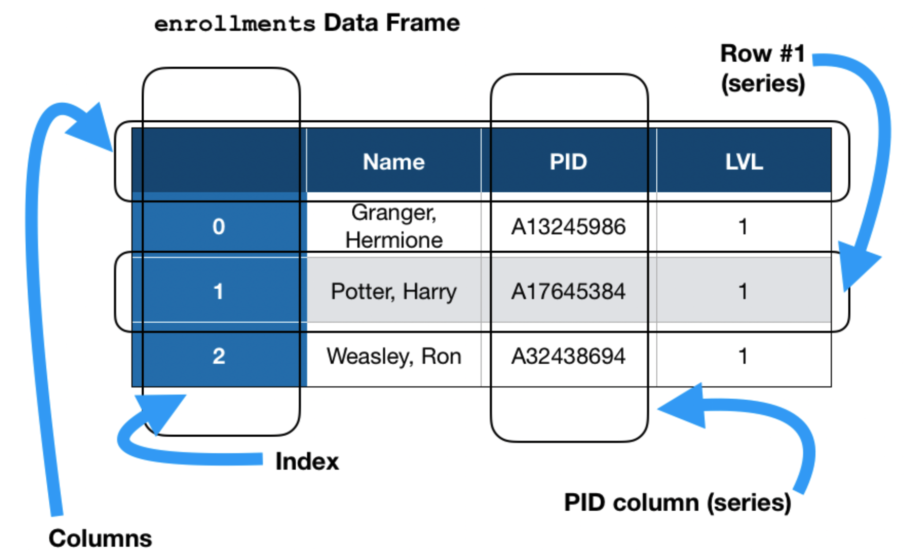A DataFrame you'll see in Lab 1.

Importing pandas and related libraries

pandas is almost always imported in conjunction with numpy.

import pandas as pd
import numpy as np

Example: Dog Breeds (woof!) 🐶

The dataset we'll work comes from the American Kennel Club. Here's a cool plot made using our dataset.

# You'll see the Path(...) / subpath syntax a lot.
# It creates the correct path to your file, 
# whether you're using Windows, macOS, or Linux.
dog_path = Path('data') / 'dogs43.csv'
dogs = pd.read_csv(dog_path)
dogs

	breed	kind	lifetime_cost	longevity	size	weight	height
0	Brittany	sporting	22589.0	12.92	medium	35.0	19.0
1	Cairn Terrier	terrier	21992.0	13.84	small	14.0	10.0
2	English Cocker Spaniel	sporting	18993.0	11.66	medium	30.0	16.0
...	...	...	...	...	...	...	...
40	Bullmastiff	working	13936.0	7.57	large	115.0	25.5
41	Mastiff	working	13581.0	6.50	large	175.0	30.0
42	Saint Bernard	working	20022.0	7.78	large	155.0	26.5

43 rows × 7 columns

Review: head, tail, shape, index, get, and sort_values

To extract the first or last few rows of a DataFrame, use the head or tail methods.

dogs.head(3)

	breed	kind	lifetime_cost	longevity	size	weight	height
0	Brittany	sporting	22589.0	12.92	medium	35.0	19.0
1	Cairn Terrier	terrier	21992.0	13.84	small	14.0	10.0
2	English Cocker Spaniel	sporting	18993.0	11.66	medium	30.0	16.0

dogs.tail(2)

	breed	kind	lifetime_cost	longevity	size	weight	height
41	Mastiff	working	13581.0	6.50	large	175.0	30.0
42	Saint Bernard	working	20022.0	7.78	large	155.0	26.5

The shape attribute returns the DataFrame's number of rows and columns.

dogs.shape

(43, 7)

# The default index of a DataFrame is 0, 1, 2, 3, ...
dogs.index

RangeIndex(start=0, stop=43, step=1)

We know that we can use .get() to select out a column or multiple columns...

dogs.get('breed')

0                   Brittany
1              Cairn Terrier
2     English Cocker Spaniel
               ...          
40               Bullmastiff
41                   Mastiff
42             Saint Bernard
Name: breed, Length: 43, dtype: object

dogs.get(['breed', 'kind', 'longevity'])

	breed	kind	longevity
0	Brittany	sporting	12.92
1	Cairn Terrier	terrier	13.84
2	English Cocker Spaniel	sporting	11.66
...	...	...	...
40	Bullmastiff	working	7.57
41	Mastiff	working	6.50
42	Saint Bernard	working	7.78

43 rows × 3 columns

Most people don't use .get in practice; we'll see the more common technique in a few slides.

And lastly, remember that to sort by a column, use the sort_values method. Like most DataFrame and Series methods, sort_values returns a new DataFrame, and doesn't modify the original.

# Note that the index is no longer 0, 1, 2, ...!
dogs.sort_values('height', ascending=False)

	breed	kind	lifetime_cost	longevity	size	weight	height
41	Mastiff	working	13581.0	6.50	large	175.0	30.0
36	Borzoi	hound	16176.0	9.08	large	82.5	28.0
34	Newfoundland	working	19351.0	9.32	large	125.0	27.0
...	...	...	...	...	...	...	...
29	Dandie Dinmont Terrier	terrier	21633.0	12.17	small	21.0	9.0
14	Maltese	toy	19084.0	12.25	small	5.0	9.0
8	Chihuahua	toy	26250.0	16.50	small	5.5	5.0

43 rows × 7 columns

# This sorts by 'height', 
# then breaks ties by 'longevity'.
# Note the difference in the last three rows between
# this DataFrame and the one above.
dogs.sort_values(['height', 'longevity'],
                 ascending=False)

	breed	kind	lifetime_cost	longevity	size	weight	height
41	Mastiff	working	13581.0	6.50	large	175.0	30.0
36	Borzoi	hound	16176.0	9.08	large	82.5	28.0
34	Newfoundland	working	19351.0	9.32	large	125.0	27.0
...	...	...	...	...	...	...	...
14	Maltese	toy	19084.0	12.25	small	5.0	9.0
29	Dandie Dinmont Terrier	terrier	21633.0	12.17	small	21.0	9.0
8	Chihuahua	toy	26250.0	16.50	small	5.5	5.0

43 rows × 7 columns

Note that dogs is not the DataFrame above. To save our changes, we'd need to say something like dogs = dogs.sort_values....

dogs

	breed	kind	lifetime_cost	longevity	size	weight	height
0	Brittany	sporting	22589.0	12.92	medium	35.0	19.0
1	Cairn Terrier	terrier	21992.0	13.84	small	14.0	10.0
2	English Cocker Spaniel	sporting	18993.0	11.66	medium	30.0	16.0
...	...	...	...	...	...	...	...
40	Bullmastiff	working	13936.0	7.57	large	115.0	25.5
41	Mastiff	working	13581.0	6.50	large	175.0	30.0
42	Saint Bernard	working	20022.0	7.78	large	155.0	26.5

43 rows × 7 columns

Setting the index

Think of each row's index as its unique identifier or name. Often, we like to set the index of a DataFrame to a unique identifier if we have one available. We can do so with the set_index method.

dogs.set_index('breed')

	kind	lifetime_cost	longevity	size	weight	height
breed
Brittany	sporting	22589.0	12.92	medium	35.0	19.0
Cairn Terrier	terrier	21992.0	13.84	small	14.0	10.0
English Cocker Spaniel	sporting	18993.0	11.66	medium	30.0	16.0
...	...	...	...	...	...	...
Bullmastiff	working	13936.0	7.57	large	115.0	25.5
Mastiff	working	13581.0	6.50	large	175.0	30.0
Saint Bernard	working	20022.0	7.78	large	155.0	26.5

43 rows × 6 columns

# The above cell didn't involve an assignment statement,
# so dogs was unchanged.
dogs

	breed	kind	lifetime_cost	longevity	size	weight	height
0	Brittany	sporting	22589.0	12.92	medium	35.0	19.0
1	Cairn Terrier	terrier	21992.0	13.84	small	14.0	10.0
2	English Cocker Spaniel	sporting	18993.0	11.66	medium	30.0	16.0
...	...	...	...	...	...	...	...
40	Bullmastiff	working	13936.0	7.57	large	115.0	25.5
41	Mastiff	working	13581.0	6.50	large	175.0	30.0
42	Saint Bernard	working	20022.0	7.78	large	155.0	26.5

43 rows × 7 columns

# By reassigning dogs, our changes will persist.
dogs = dogs.set_index('breed')
dogs

	kind	lifetime_cost	longevity	size	weight	height
breed
Brittany	sporting	22589.0	12.92	medium	35.0	19.0
Cairn Terrier	terrier	21992.0	13.84	small	14.0	10.0
English Cocker Spaniel	sporting	18993.0	11.66	medium	30.0	16.0
...	...	...	...	...	...	...
Bullmastiff	working	13936.0	7.57	large	115.0	25.5
Mastiff	working	13581.0	6.50	large	175.0	30.0
Saint Bernard	working	20022.0	7.78	large	155.0	26.5

43 rows × 6 columns

# There used to be 7 columns, but now there are only 6!
dogs.shape

(43, 6)

Question 🤔 (Answer at `lec02-query`)

Ask ChatGPT:

• To explain what happens if you have duplicate values in a column and use set_index() on it.

💡 Pro-Tip: Displaying more rows/columns

Sometimes, you just want pandas to display a lot of rows and columns. You can use this helper function to do that:

from IPython.display import display
def display_df(df, rows=pd.options.display.max_rows, cols=pd.options.display.max_columns):
    """Displays n rows and cols from df."""
    with pd.option_context("display.max_rows", rows,
                           "display.max_columns", cols):
        display(df)

display_df(dogs.sort_values('weight', ascending=False),
           rows=43)

	kind	lifetime_cost	longevity	size	weight	height
breed
Mastiff	working	13581.0	6.50	large	175.0	30.00
Saint Bernard	working	20022.0	7.78	large	155.0	26.50
Newfoundland	working	19351.0	9.32	large	125.0	27.00
Bullmastiff	working	13936.0	7.57	large	115.0	25.50
Bloodhound	hound	13824.0	6.75	large	85.0	25.00
Borzoi	hound	16176.0	9.08	large	82.5	28.00
Alaskan Malamute	working	21986.0	10.67	large	80.0	24.00
Rhodesian Ridgeback	hound	16530.0	9.10	large	77.5	25.50
Giant Schnauzer	working	26686.0	10.00	large	77.5	25.50
Clumber Spaniel	sporting	18084.0	10.00	medium	70.0	18.50
Labrador Retriever	sporting	21299.0	12.04	medium	67.5	23.00
Chesapeake Bay Retriever	sporting	16697.0	9.48	large	67.5	23.50
Irish Setter	sporting	20323.0	11.63	large	65.0	26.00
German Shorthaired Pointer	sporting	25842.0	11.46	large	62.5	24.00
Gordon Setter	sporting	19605.0	11.10	large	62.5	25.00
Bull Terrier	terrier	18490.0	10.21	medium	60.0	21.50
Golden Retriever	sporting	21447.0	12.04	medium	60.0	22.75
Pointer	sporting	24445.0	12.42	large	59.5	25.50
Afghan Hound	hound	24077.0	11.92	large	55.0	26.00
Siberian Husky	working	22049.0	12.58	medium	47.5	21.75
English Springer Spaniel	sporting	21946.0	12.54	medium	45.0	19.50
Kerry Blue Terrier	terrier	17240.0	9.40	medium	36.5	18.50
Brittany	sporting	22589.0	12.92	medium	35.0	19.00
Staffordshire Bull Terrier	terrier	21650.0	12.05	medium	31.0	15.00
English Cocker Spaniel	sporting	18993.0	11.66	medium	30.0	16.00
Pembroke Welsh Corgi	herding	23978.0	12.25	small	26.0	11.00
Cocker Spaniel	sporting	24330.0	12.50	small	25.0	14.50
Tibetan Terrier	non-sporting	20336.0	12.31	small	24.0	15.50
Basenji	hound	22096.0	13.58	medium	23.0	16.50
Shetland Sheepdog	herding	21006.0	12.53	small	22.0	14.50
Dandie Dinmont Terrier	terrier	21633.0	12.17	small	21.0	9.00
Scottish Terrier	terrier	17525.0	10.69	small	20.0	10.00
Pug	toy	18527.0	11.00	medium	16.0	16.00
Miniature Schnauzer	terrier	20087.0	11.81	small	15.5	13.00
Cavalier King Charles Spaniel	toy	18639.0	11.29	small	15.5	12.50
Lhasa Apso	non-sporting	22031.0	13.92	small	15.0	10.50
Cairn Terrier	terrier	21992.0	13.84	small	14.0	10.00
Shih Tzu	toy	21152.0	13.20	small	12.5	9.75
Tibetan Spaniel	non-sporting	25549.0	14.42	small	12.0	10.00
Norfolk Terrier	terrier	24308.0	13.07	small	12.0	9.50
English Toy Spaniel	toy	17521.0	10.10	small	11.0	10.00
Chihuahua	toy	26250.0	16.50	small	5.5	5.00
Maltese	toy	19084.0	12.25	small	5.0	9.00

Selecting columns

Selecting columns in babypandas 👶🐼

• In babypandas, you selected columns using the .get method.
• .get also works in pandas, but it is not idiomatic – people don't usually use it.

dogs

	kind	lifetime_cost	longevity	size	weight	height
breed
Brittany	sporting	22589.0	12.92	medium	35.0	19.0
Cairn Terrier	terrier	21992.0	13.84	small	14.0	10.0
English Cocker Spaniel	sporting	18993.0	11.66	medium	30.0	16.0
...	...	...	...	...	...	...
Bullmastiff	working	13936.0	7.57	large	115.0	25.5
Mastiff	working	13581.0	6.50	large	175.0	30.0
Saint Bernard	working	20022.0	7.78	large	155.0	26.5

43 rows × 6 columns

dogs.get('size')

breed
Brittany                  medium
Cairn Terrier              small
English Cocker Spaniel    medium
                           ...  
Bullmastiff                large
Mastiff                    large
Saint Bernard              large
Name: size, Length: 43, dtype: object

# This doesn't error, but sometimes we'd like it to.
dogs.get('size oops!')

Selecting columns with []

• The standard way to select a column in pandas is by using the [] operator.
• Specifying a column name returns the column as a Series.
• Specifying a list of column names returns a DataFrame.

dogs

	kind	lifetime_cost	longevity	size	weight	height
breed
Brittany	sporting	22589.0	12.92	medium	35.0	19.0
Cairn Terrier	terrier	21992.0	13.84	small	14.0	10.0
English Cocker Spaniel	sporting	18993.0	11.66	medium	30.0	16.0
...	...	...	...	...	...	...
Bullmastiff	working	13936.0	7.57	large	115.0	25.5
Mastiff	working	13581.0	6.50	large	175.0	30.0
Saint Bernard	working	20022.0	7.78	large	155.0	26.5

43 rows × 6 columns

# Returns a Series.
dogs['kind']

breed
Brittany                  sporting
Cairn Terrier              terrier
English Cocker Spaniel    sporting
                            ...   
Bullmastiff                working
Mastiff                    working
Saint Bernard              working
Name: kind, Length: 43, dtype: object

# Returns a DataFrame.
dogs[['kind', 'size']]

	kind	size
breed
Brittany	sporting	medium
Cairn Terrier	terrier	small
English Cocker Spaniel	sporting	medium
...	...	...
Bullmastiff	working	large
Mastiff	working	large
Saint Bernard	working	large

43 rows × 2 columns

# 🤔
dogs[['kind']]

	kind
breed
Brittany	sporting
Cairn Terrier	terrier
English Cocker Spaniel	sporting
...	...
Bullmastiff	working
Mastiff	working
Saint Bernard	working

43 rows × 1 columns

# Breeds are stored in the index, which is not a column!
dogs['breed']

---------------------------------------------------------------------------
KeyError                                  Traceback (most recent call last)
File ~/miniforge3/envs/dsc80/lib/python3.12/site-packages/pandas/core/indexes/base.py:3805, in Index.get_loc(self, key)
   3804 try:
-> 3805     return self._engine.get_loc(casted_key)
   3806 except KeyError as err:

File index.pyx:167, in pandas._libs.index.IndexEngine.get_loc()

File index.pyx:196, in pandas._libs.index.IndexEngine.get_loc()

File pandas/_libs/hashtable_class_helper.pxi:7081, in pandas._libs.hashtable.PyObjectHashTable.get_item()

File pandas/_libs/hashtable_class_helper.pxi:7089, in pandas._libs.hashtable.PyObjectHashTable.get_item()

KeyError: 'breed'

The above exception was the direct cause of the following exception:

KeyError                                  Traceback (most recent call last)
Cell In[85], line 2
      1 # Breeds are stored in the index, which is not a column!
----> 2 dogs['breed']

File ~/miniforge3/envs/dsc80/lib/python3.12/site-packages/pandas/core/frame.py:4102, in DataFrame.__getitem__(self, key)
   4100 if self.columns.nlevels > 1:
   4101     return self._getitem_multilevel(key)
-> 4102 indexer = self.columns.get_loc(key)
   4103 if is_integer(indexer):
   4104     indexer = [indexer]

File ~/miniforge3/envs/dsc80/lib/python3.12/site-packages/pandas/core/indexes/base.py:3812, in Index.get_loc(self, key)
   3807     if isinstance(casted_key, slice) or (
   3808         isinstance(casted_key, abc.Iterable)
   3809         and any(isinstance(x, slice) for x in casted_key)
   3810     ):
   3811         raise InvalidIndexError(key)
-> 3812     raise KeyError(key) from err
   3813 except TypeError:
   3814     # If we have a listlike key, _check_indexing_error will raise
   3815     #  InvalidIndexError. Otherwise we fall through and re-raise
   3816     #  the TypeError.
   3817     self._check_indexing_error(key)

KeyError: 'breed'

dogs.index

Index(['Brittany', 'Cairn Terrier', 'English Cocker Spaniel', 'Cocker Spaniel',
       'Shetland Sheepdog', 'Siberian Husky', 'Lhasa Apso',
       'Miniature Schnauzer', 'Chihuahua', 'English Springer Spaniel',
       'German Shorthaired Pointer', 'Pointer', 'Tibetan Spaniel',
       'Labrador Retriever', 'Maltese', 'Shih Tzu', 'Irish Setter',
       'Golden Retriever', 'Chesapeake Bay Retriever', 'Tibetan Terrier',
       'Gordon Setter', 'Pug', 'Norfolk Terrier', 'English Toy Spaniel',
       'Cavalier King Charles Spaniel', 'Basenji',
       'Staffordshire Bull Terrier', 'Pembroke Welsh Corgi', 'Clumber Spaniel',
       'Dandie Dinmont Terrier', 'Giant Schnauzer', 'Scottish Terrier',
       'Kerry Blue Terrier', 'Afghan Hound', 'Newfoundland',
       'Rhodesian Ridgeback', 'Borzoi', 'Bull Terrier', 'Alaskan Malamute',
       'Bloodhound', 'Bullmastiff', 'Mastiff', 'Saint Bernard'],
      dtype='object', name='breed')

Useful Series methods

There are a variety of useful methods that work on Series. You can see the entire list here. Many methods that work on a Series will also work on DataFrames, as we'll soon see.

dogs

	kind	lifetime_cost	longevity	size	weight	height
breed
Brittany	sporting	22589.0	12.92	medium	35.0	19.0
Cairn Terrier	terrier	21992.0	13.84	small	14.0	10.0
English Cocker Spaniel	sporting	18993.0	11.66	medium	30.0	16.0
...	...	...	...	...	...	...
Bullmastiff	working	13936.0	7.57	large	115.0	25.5
Mastiff	working	13581.0	6.50	large	175.0	30.0
Saint Bernard	working	20022.0	7.78	large	155.0	26.5

43 rows × 6 columns

# What are the unique kinds of dogs?
dogs['kind'].unique()

array(['sporting', 'terrier', 'herding', 'working', 'non-sporting', 'toy',
       'hound'], dtype=object)

# How many unique kinds of dogs are there?
dogs['kind'].nunique()

7

# What's the distribution of kinds?
dogs['kind'].value_counts()

kind
sporting        12
terrier          8
working          7
toy              6
hound            5
non-sporting     3
herding          2
Name: count, dtype: int64

# What's the mean of the 'longevity' column?
dogs['longevity'].mean()

np.float64(11.340697674418605)

# Tell me more about the 'weight' column.
dogs['weight'].describe()

count     43.00
mean      49.35
std       39.42
          ...  
50%       36.50
75%       67.50
max      175.00
Name: weight, Length: 8, dtype: float64

# Sort the 'lifetime_cost' column. Note that here we're using sort_values on a Series, not a DataFrame!
dogs['lifetime_cost'].sort_values()

breed
Mastiff                       13581.0
Bloodhound                    13824.0
Bullmastiff                   13936.0
                               ...   
German Shorthaired Pointer    25842.0
Chihuahua                     26250.0
Giant Schnauzer               26686.0
Name: lifetime_cost, Length: 43, dtype: float64

# Gives us the index of the largest value, not the largest value itself.
dogs['lifetime_cost'].idxmax()

'Giant Schnauzer'

Selecting subsets of rows (and columns)

Use loc to slice rows and columns using labels

You saw slicing in DSC 20.

loc works similarly to slicing 2D arrays, but it uses row labels and column labels, not positions.

dogs.loc['Pug']

kind                 toy
lifetime_cost    18527.0
longevity           11.0
size              medium
weight              16.0
height              16.0
Name: Pug, dtype: object

# The first argument is the row label.
#        ↓
dogs.loc['Pug', 'longevity']
#                  ↑
# The second argument is the column label.

np.float64(11.0)

As an aside, loc is not a method – it's an indexer.

type(dogs.loc)

pandas.core.indexing._LocIndexer

type(dogs.sort_values)

method

.loc is flexible 🧘

You can provide a sequence (list, array, Series) as either argument to .loc.

dogs

	kind	lifetime_cost	longevity	size	weight	height
breed
Brittany	sporting	22589.0	12.92	medium	35.0	19.0
Cairn Terrier	terrier	21992.0	13.84	small	14.0	10.0
English Cocker Spaniel	sporting	18993.0	11.66	medium	30.0	16.0
...	...	...	...	...	...	...
Bullmastiff	working	13936.0	7.57	large	115.0	25.5
Mastiff	working	13581.0	6.50	large	175.0	30.0
Saint Bernard	working	20022.0	7.78	large	155.0	26.5

43 rows × 6 columns

dogs.loc[['Cocker Spaniel', 'Labrador Retriever'], 'size']

breed
Cocker Spaniel         small
Labrador Retriever    medium
Name: size, dtype: object

dogs.loc[['Cocker Spaniel', 'Labrador Retriever'], ['kind', 'size', 'height']]

# Note that the 'weight' column is included!
dogs.loc[['Cocker Spaniel', 'Labrador Retriever'], 'lifetime_cost': 'weight']

dogs.loc[['Cocker Spaniel', 'Labrador Retriever'], :]

# Shortcut for the line above.
dogs.loc[['Cocker Spaniel', 'Labrador Retriever']]

Review: Querying

• As we saw in DSC 10, querying is the act of selecting rows in a DataFrame that satisfy certain condition(s).
• Comparisons with arrays (or Series) result in Boolean arrays (or Series).
• We can use comparisons along with the loc operator to filter a DataFrame.

dogs

dogs.loc[dogs['weight'] < 10]

dogs.loc[dogs.index.str.contains('Retriever')]

# Because querying is so common, there's a shortcut:
dogs[dogs.index.str.contains('Retriever')]

# Empty DataFrame – not an error!
dogs.loc[dogs['kind'] == 'beaver']

Note that because we set the index to 'breed' earlier, we can select rows based on dog breeds without having to query.

dogs

# Series!
dogs.loc['Maltese']

If 'breed' was instead a column, then we'd need to query to access information about a particular breed.

dogs_reset = dogs.reset_index()
dogs_reset

# DataFrame!
dogs_reset[dogs_reset['breed'] == 'Maltese']

Querying with multiple conditions

Remember, you need parentheses around each condition. Also, you must use the bitwise operators & and | instead of the standard and and or keywords. pandas makes weird decisions sometimes!

dogs

dogs[(dogs['weight'] < 20) & (dogs['kind'] == 'terrier')]

💡 Pro-Tip: Using .query

.query is a convenient way to query, since you don't need parentheses and you can use the and and or keywords.

dogs

dogs.query('weight < 20 and kind == "terrier"')

dogs.query('kind in ["sporting", "terrier"] and lifetime_cost < 20000')

Question 🤔 (Answer at `lec02-index`)

Ask ChatGPT:

• To explain when you would use .query() instead of .loc[] or the other way around.

Don't forget iloc!

• iloc stands for "integer location."
• iloc is like loc, but it selects rows and columns based off of integer positions only, just like with 2D arrays.

dogs

dogs.iloc[1:15, :-2]

iloc is often most useful when we sort first. For instance, to find the weight of the longest-living dog breed in the dataset:

dogs.sort_values('longevity', ascending=False)['weight'].iloc[0]

# Finding the breed itself involves sorting, but not iloc.
dogs.sort_values('longevity', ascending=False).index[0]

More practice

Consider the DataFrame below.

jack = pd.DataFrame({1: ['fee', 'fi'], 
                     '1': ['fo', 'fum']})
jack

For each of the following pieces of code, predict what the output will be. Then, uncomment the line of code and see for yourself. We may not be able to cover these all in class; if so, make sure to try them on your own. Here's a Pandas Tutor link to visualize these!

# jack[1]

# jack[[1]]

# jack['1']

# jack[[1, 1]]

# jack.loc[1]

# jack.loc[jack[1] == 'fo']

# jack[1, ['1', 1]]

# jack.loc[1,1]

Questions? 🤔

What questions do you have?

We will probably have to end lecture here.

Adding and modifying columns

Adding and modifying columns, using a copy

• To add a new column to a DataFrame, use the assign method.
  • To change the values in a column, add a new column with the same name as the existing column.
• Like most pandas methods, assign returns a new DataFrame.
  • Pro ✅: This doesn't inadvertently change any existing variables.
  • Con ❌: It is not very space efficient, as it creates a new copy each time it is called.

dogs.assign(cost_per_year=dogs['lifetime_cost'] / dogs['longevity'])

dogs

💡 Pro-Tip: Method chaining

Chain methods together instead of writing long, hard-to-read lines.

# Finds the rows corresponding to the five cheapest to own breeds on a per-year basis.
(dogs
 .assign(cost_per_year=dogs['lifetime_cost'] / dogs['longevity'])
 .sort_values('cost_per_year')
 .iloc[:5]
)

💡 Pro-Tip: assign for column names with special characters

You can also use assign when the desired column name has spaces (and other special characters) by unpacking a dictionary:

dogs.assign(**{'cost per year 💵': dogs['lifetime_cost'] / dogs['longevity']})

Adding and modifying columns, in-place

• You can assign a new column to a DataFrame in-place using [].
  • This works like dictionary assignment.
  • This modifies the underlying DataFrame, unlike assign, which returns a new DataFrame.
• This is the more "common" way of adding/modifying columns.
  • ⚠️ Warning: Exercise caution when using this approach, since this approach changes the values of existing variables.

# By default, .copy() returns a deep copy of the object it is called on,
# meaning that if you change the copy the original remains unmodified.
dogs_copy = dogs.copy()
dogs_copy.head(2)

dogs_copy['cost_per_year'] = dogs_copy['lifetime_cost'] / dogs_copy['longevity']
dogs_copy

Note that we never reassigned dogs_copy in the cell above – that is, we never wrote dogs_copy = ... – though it was still modified.

Mutability

DataFrames, like lists, arrays, and dictionaries, are mutable. As you learned in DSC 20, this means that they can be modified after being created. (For instance, the list .append method mutates in-place.)

Not only does this explain the behavior on the previous slide, but it also explains the following:

dogs_copy

def cost_in_thousands():
    dogs_copy['lifetime_cost'] = dogs_copy['lifetime_cost'] / 1000

# What happens when we run this twice?
cost_in_thousands()

dogs_copy

⚠️ Avoid mutation when possible

Note that dogs_copy was modified, even though we didn't reassign it! These unintended consequences can influence the behavior of test cases on labs and projects, among other things!

To avoid this, it's a good idea to avoid mutation when possible. If you must use mutation, include df = df.copy() as the first line in functions that take DataFrames as input.

Also, some methods let you use the inplace=True argument to mutate the original. Don't use this argument, since future pandas releases plan to remove it.

pandas and numpy

pandas is built upon numpy!

• A Series in pandas is a numpy array with an index.
• A DataFrame is like a dictionary of columns, each of which is a numpy array.
• Many operations in pandas are fast because they use numpy's implementations, which are written in fast languages like C.
• If you need access the array underlying a DataFrame or Series, use the to_numpy method.

dogs['lifetime_cost']

dogs['lifetime_cost'].to_numpy()

pandas data types

• Each Series (column) has a numpy data type, which refers to the type of the values stored within. Access it using the dtypes attribute.
• A column's data type determines which operations can be applied to it.
• pandas tries to guess the correct data types for a given DataFrame, and is often wrong.
  • This can lead to incorrect calculations and poor memory/time performance.
• As a result, you will often need to explicitly convert between data types.

dogs

dogs.dtypes

pandas data types

Notice that Python str types are object types in numpy and pandas.

Pandas dtype	Python type	NumPy type	SQL type	Usage
int64	int	int_, int8,...,int64, uint8,...,uint64	INT, BIGINT	Integer numbers
float64	float	float_, float16, float32, float64	FLOAT	Floating point numbers
bool	bool	bool_	BOOL	True/False values
datetime64 or Timestamp	datetime.datetime	datetime64	DATETIME	Date and time values
timedelta64 or Timedelta	datetime.timedelta	timedelta64	NA	Differences between two datetimes
category	NA	NA	ENUM	Finite list of text values
object	str	string, unicode	NA	Text
object	NA	object	NA	Mixed types

This article details how pandas stores different data types under the hood.

This article explains how numpy/pandas int64 operations differ from vanilla int operations.

Type conversion

You can change the data type of a Series using the .astype Series method.

For example, we can change the data type of the 'lifetime_cost' column in dogs to be uint32:

dogs

# Gives the types as well as the space taken up by the DataFrame.
dogs.info()

dogs['lifetime_cost'] = dogs['lifetime_cost'].astype('uint32')

Now, the DataFrame takes up less space! This may be insignificant in our DataFrame, but makes a difference when working with larger datasets.

dogs.info()

💡 Pro-Tip: Setting dtypes in read_csv

Usually, we prefer to set the correct dtypes in read_csv, since it can help pandas load in files more quickly:

dog_path

dogs = pd.read_csv(dog_path, dtype={'lifetime_cost': 'uint32'})
dogs

dogs.dtypes

Axes

• The rows and columns of a DataFrame are both stored as Series.
• The axis specifies the direction of a slice of a DataFrame.

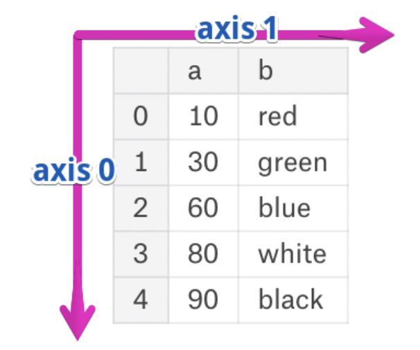
• Axis 0 refers to the index (rows).
• Axis 1 refers to the columns.
• These are the same axes definitions that 2D numpy arrays have!

DataFrame methods with axis

• Many Series methods work on DataFrames.
• In such cases, the DataFrame method usually applies the Series method to every row or column.
• Many of these methods accept an axis argument; the default is usually axis=0.

dogs

# Max element in each column.
dogs.max()

# Max element in each row – throws an error since there are different types in each row.
# dogs.max(axis=1)

# The number of unique values in each column.
dogs.nunique()

# describe doesn't accept an axis argument; it works on every numeric column in the DataFrame it is called on.
dogs.describe()

Exercise

Pick a dog breed that you personally like or know the name of. Then:

• Try to find a few other dog breeds that are similar in weight to yours in all_dogs.
• Which similar breeds have the lowest and highest 'lifetime_cost'? 'intelligence_rank'?
• Are there any similar breeds that you haven't heard of before?

For fun, look up these dog breeds on the AKC website to see what they look like!

all_dogs = pd.read_csv(Path('data') / 'all_dogs.csv')
all_dogs

# Your code goes here.

Summary, next time

Summary

• pandas is the library for tabular data manipulation in Python.
• There are three key data structures in pandas: DataFrame, Series, and Index.
• Refer to the lecture notebook and the pandas documentation for tips.
• pandas relies heavily on numpy. An understanding of how data types work in both will allow you to write more efficient and bug-free code.
• Series and DataFrames share many methods (refer to the pandas documentation for more details).
• Most pandas methods return copies of Series/DataFrames. Be careful when using techniques that modify values in-place.
• Next time: groupby and data granularity.