from dsc80_utils import *
def show_paradox_slides():
src = 'https://docs.google.com/presentation/d/e/2PACX-1vSbFSaxaYZ0NcgrgqZLvjhkjX-5MQzAITWAsEFZHnix3j1c0qN8Vd1rogTAQP7F7Nf5r-JWExnGey7h/embed?start=false&rm=minimal'
width = 960
height = 569
display(IFrame(src, width, height))
# Pandas Tutor setup
!pip install pandas-tutor
%reload_ext pandas_tutor
%set_pandas_tutor_options {"maxDisplayCols": 8, "nohover": True, "projectorMode": True}
import warnings
warnings.simplefilter(action='ignore', category=FutureWarning)
Requirement already satisfied: pandas-tutor in /Users/tauhidur/miniforge3/envs/dsc80/lib/python3.12/site-packages (2.0.4) Requirement already satisfied: pandas>=1.3 in /Users/tauhidur/miniforge3/envs/dsc80/lib/python3.12/site-packages (from pandas-tutor) (2.2.3) Requirement already satisfied: mypy-extensions==0.4.3 in /Users/tauhidur/miniforge3/envs/dsc80/lib/python3.12/site-packages (from pandas-tutor) (0.4.3) Requirement already satisfied: typing-extensions<5.0,>=4.1 in /Users/tauhidur/miniforge3/envs/dsc80/lib/python3.12/site-packages (from pandas-tutor) (4.12.2) Requirement already satisfied: numpy>=1.26.0 in /Users/tauhidur/miniforge3/envs/dsc80/lib/python3.12/site-packages (from pandas>=1.3->pandas-tutor) (2.1.1) Requirement already satisfied: python-dateutil>=2.8.2 in /Users/tauhidur/miniforge3/envs/dsc80/lib/python3.12/site-packages (from pandas>=1.3->pandas-tutor) (2.9.0.post0) Requirement already satisfied: pytz>=2020.1 in /Users/tauhidur/miniforge3/envs/dsc80/lib/python3.12/site-packages (from pandas>=1.3->pandas-tutor) (2024.1) Requirement already satisfied: tzdata>=2022.7 in /Users/tauhidur/miniforge3/envs/dsc80/lib/python3.12/site-packages (from pandas>=1.3->pandas-tutor) (2025.1) Requirement already satisfied: six>=1.5 in /Users/tauhidur/miniforge3/envs/dsc80/lib/python3.12/site-packages (from python-dateutil>=2.8.2->pandas>=1.3->pandas-tutor) (1.17.0)
Agenda
- Pivot tables.
- Distributions.
- Simpson's paradox.
- Merging.
- Many-to-one & many-to-many joins.
- Transforming.
- The price of
apply.
- The price of
Grouping with multiple columns
When we group with multiple columns, one group is created for every unique combination of elements in the specified columns.
import seaborn as sns
penguins = sns.load_dataset('penguins').dropna()
penguins
| species | island | bill_length_mm | bill_depth_mm | flipper_length_mm | body_mass_g | sex | |
|---|---|---|---|---|---|---|---|
| 0 | Adelie | Torgersen | 39.1 | 18.7 | 181.0 | 3750.0 | Male |
| 1 | Adelie | Torgersen | 39.5 | 17.4 | 186.0 | 3800.0 | Female |
| 2 | Adelie | Torgersen | 40.3 | 18.0 | 195.0 | 3250.0 | Female |
| ... | ... | ... | ... | ... | ... | ... | ... |
| 341 | Gentoo | Biscoe | 50.4 | 15.7 | 222.0 | 5750.0 | Male |
| 342 | Gentoo | Biscoe | 45.2 | 14.8 | 212.0 | 5200.0 | Female |
| 343 | Gentoo | Biscoe | 49.9 | 16.1 | 213.0 | 5400.0 | Male |
333 rows × 7 columns
species_and_island = (
penguins
.groupby(['species', 'island'])
[['bill_length_mm', 'body_mass_g']]
.mean()
)
species_and_island
| bill_length_mm | body_mass_g | ||
|---|---|---|---|
| species | island | ||
| Adelie | Biscoe | 38.98 | 3709.66 |
| Dream | 38.52 | 3701.36 | |
| Torgersen | 39.04 | 3708.51 | |
| Chinstrap | Dream | 48.83 | 3733.09 |
| Gentoo | Biscoe | 47.57 | 5092.44 |
Grouping and indexes
- The
groupbymethod creates an index based on the specified columns. - When grouping by multiple columns, the resulting DataFrame has a
MultiIndex. - Advice: When working with a
MultiIndex, usereset_indexor setas_index=Falseingroupby.
species_and_island
| bill_length_mm | body_mass_g | ||
|---|---|---|---|
| species | island | ||
| Adelie | Biscoe | 38.98 | 3709.66 |
| Dream | 38.52 | 3701.36 | |
| Torgersen | 39.04 | 3708.51 | |
| Chinstrap | Dream | 48.83 | 3733.09 |
| Gentoo | Biscoe | 47.57 | 5092.44 |
species_and_island['body_mass_g']
species island
Adelie Biscoe 3709.66
Dream 3701.36
Torgersen 3708.51
Chinstrap Dream 3733.09
Gentoo Biscoe 5092.44
Name: body_mass_g, dtype: float64
species_and_island.loc['Adelie']
| bill_length_mm | body_mass_g | |
|---|---|---|
| island | ||
| Biscoe | 38.98 | 3709.66 |
| Dream | 38.52 | 3701.36 |
| Torgersen | 39.04 | 3708.51 |
species_and_island.loc[('Adelie', 'Torgersen')]
bill_length_mm 39.04 body_mass_g 3708.51 Name: (Adelie, Torgersen), dtype: float64
species_and_island.reset_index()
| species | island | bill_length_mm | body_mass_g | |
|---|---|---|---|---|
| 0 | Adelie | Biscoe | 38.98 | 3709.66 |
| 1 | Adelie | Dream | 38.52 | 3701.36 |
| 2 | Adelie | Torgersen | 39.04 | 3708.51 |
| 3 | Chinstrap | Dream | 48.83 | 3733.09 |
| 4 | Gentoo | Biscoe | 47.57 | 5092.44 |
(penguins
.groupby(['species', 'island'], as_index=False)
[['bill_length_mm', 'body_mass_g']]
.mean()
)
| species | island | bill_length_mm | body_mass_g | |
|---|---|---|---|---|
| 0 | Adelie | Biscoe | 38.98 | 3709.66 |
| 1 | Adelie | Dream | 38.52 | 3701.36 |
| 2 | Adelie | Torgersen | 39.04 | 3708.51 |
| 3 | Chinstrap | Dream | 48.83 | 3733.09 |
| 4 | Gentoo | Biscoe | 47.57 | 5092.44 |
baby_path = Path('data') / 'baby.csv'
baby = pd.read_csv(baby_path)
baby
| Name | Sex | Count | Year | |
|---|---|---|---|---|
| 0 | Liam | M | 20456 | 2022 |
| 1 | Noah | M | 18621 | 2022 |
| 2 | Olivia | F | 16573 | 2022 |
| ... | ... | ... | ... | ... |
| 2085155 | Wright | M | 5 | 1880 |
| 2085156 | York | M | 5 | 1880 |
| 2085157 | Zachariah | M | 5 | 1880 |
2085158 rows × 4 columns
# Your code goes here.
Pivot tables using the pivot_table method
Pivot tables: an extension of grouping
Pivot tables are a compact way to display tables for humans to read:
| Sex | F | M |
|---|---|---|
| Year | ||
| 2018 | 1698373 | 1813377 |
| 2019 | 1675139 | 1790682 |
| 2020 | 1612393 | 1721588 |
| 2021 | 1635800 | 1743913 |
| 2022 | 1628730 | 1733166 |
- Notice that each value in the table is a sum over the counts, split by year and sex.
- You can think of pivot tables as grouping using two columns, then "pivoting" one of the group labels into columns.
pivot_table
The pivot_table DataFrame method aggregates a DataFrame using two columns. To use it:
df.pivot_table(index=index_col,
columns=columns_col,
values=values_col,
aggfunc=func)
The resulting DataFrame will have:
- One row for every unique value in
index_col. - One column for every unique value in
columns_col. - Values determined by applying
funcon values invalues_col.
penguins.pivot_table(
index='species',
columns='island',
values='bill_length_mm', # Choice of column here doesn't actually matter!
aggfunc='count',
)
| island | Biscoe | Dream | Torgersen |
|---|---|---|---|
| species | |||
| Adelie | 44.0 | 55.0 | 47.0 |
| Chinstrap | NaN | 68.0 | NaN |
| Gentoo | 119.0 | NaN | NaN |
Note that there is a NaN at the intersection of 'Biscoe' and 'Chinstrap', because there were no Chinstrap penguins on Biscoe Island.
We can either use the fillna method afterwards or the fill_value argument to fill in NaNs.
penguins.pivot_table(
index='species',
columns='island',
values='bill_length_mm',
aggfunc='count',
fill_value=0,
)
| island | Biscoe | Dream | Torgersen |
|---|---|---|---|
| species | |||
| Adelie | 44 | 55 | 47 |
| Chinstrap | 0 | 68 | 0 |
| Gentoo | 119 | 0 | 0 |
# Look at the similarity to the snippet above!
(penguins
.groupby(['species', 'island'])
[['bill_length_mm']]
.count()
)
| bill_length_mm | ||
|---|---|---|
| species | island | |
| Adelie | Biscoe | 44 |
| Dream | 55 | |
| Torgersen | 47 | |
| Chinstrap | Dream | 68 |
| Gentoo | Biscoe | 119 |
Distributions
Example: Palmer Penguins
penguins = sns.load_dataset('penguins').dropna()
penguins
| species | island | bill_length_mm | bill_depth_mm | flipper_length_mm | body_mass_g | sex | |
|---|---|---|---|---|---|---|---|
| 0 | Adelie | Torgersen | 39.1 | 18.7 | 181.0 | 3750.0 | Male |
| 1 | Adelie | Torgersen | 39.5 | 17.4 | 186.0 | 3800.0 | Female |
| 2 | Adelie | Torgersen | 40.3 | 18.0 | 195.0 | 3250.0 | Female |
| ... | ... | ... | ... | ... | ... | ... | ... |
| 341 | Gentoo | Biscoe | 50.4 | 15.7 | 222.0 | 5750.0 | Male |
| 342 | Gentoo | Biscoe | 45.2 | 14.8 | 212.0 | 5200.0 | Female |
| 343 | Gentoo | Biscoe | 49.9 | 16.1 | 213.0 | 5400.0 | Male |
333 rows × 7 columns
Let's start by using the pivot_table method to recreate the DataFrame shown below.
| sex | Female | Male |
|---|---|---|
| species | ||
| Adelie | 73 | 73 |
| Chinstrap | 34 | 34 |
| Gentoo | 58 | 61 |
Joint distribution
When using aggfunc='count', a pivot table describes the joint distribution of two categorical variables. This is also called a contingency table.
counts = penguins.pivot_table(
index='species',
columns='sex',
values='body_mass_g',
aggfunc='size',
fill_value=0,
)
counts
| sex | Female | Male |
|---|---|---|
| species | ||
| Adelie | 73 | 73 |
| Chinstrap | 34 | 34 |
| Gentoo | 58 | 61 |
We can normalize the DataFrame by dividing by the total number of penguins. The resulting numbers can be interpreted as probabilities that a randomly selected penguin from the dataset belongs to a given combination of species and sex.
counts.sum()
sex Female 165 Male 168 dtype: int64
Marginal probabilities
If we sum over one of the axes, we can compute marginal probabilities, i.e. unconditional probabilities.
joint = counts/counts.sum().sum()
joint
| sex | Female | Male |
|---|---|---|
| species | ||
| Adelie | 0.22 | 0.22 |
| Chinstrap | 0.10 | 0.10 |
| Gentoo | 0.17 | 0.18 |
# Recall, joint.sum(axis=0) sums across the rows,
# which computes the sum of the **columns**.
joint.sum(axis=0)
sex Female 0.5 Male 0.5 dtype: float64
joint.sum(axis=1)
species Adelie 0.44 Chinstrap 0.20 Gentoo 0.36 dtype: float64
For instance, the second Series tells us that a randomly selected penguin has a 0.36 chance of being of species 'Gentoo'.
Conditional probabilities
Using counts, how might we compute conditional probabilities like $$P(\text{species } = \text{"Adelie"} \mid \text{sex } = \text{"Female"})?$$
counts
| sex | Female | Male |
|---|---|---|
| species | ||
| Adelie | 73 | 73 |
| Chinstrap | 34 | 34 |
| Gentoo | 58 | 61 |
$$\begin{align*} P(\text{species} = c \mid \text{sex} = x) &= \frac{\# \: (\text{species} = c \text{ and } \text{sex} = x)}{\# \: (\text{sex} = x)} \end{align*}$$
➡️ Click here to see more of a derivation.
$$\begin{align*} P(\text{species} = c \mid \text{sex} = x) &= \frac{P(\text{species} = c \text{ and } \text{sex} = x)}{P(\text{sex = }x)} \\ &= \frac{\frac{\# \: (\text{species } = \: c \text{ and } \text{sex } = \: x)}{N}}{\frac{\# \: (\text{sex } = \: x)}{N}} \\ &= \frac{\# \: (\text{species} = c \text{ and } \text{sex} = x)}{\# \: (\text{sex} = x)} \end{align*}$$Answer: To find conditional probabilities of 'species' given 'sex', divide by column sums. To find conditional probabilities of 'sex' given 'species', divide by row sums.
Conditional probabilities
To find conditional probabilities of 'species' given 'sex', divide by column sums. To find conditional probabilities of 'sex' given 'species', divide by row sums.
counts.sum(axis=0)
sex Female 165 Male 168 dtype: int64
The conditional distribution of 'species' given 'sex' is below. Note that in this new DataFrame, the 'Female' and 'Male' columns each sum to 1.
counts / counts.sum(axis=0)
| sex | Female | Male |
|---|---|---|
| species | ||
| Adelie | 0.44 | 0.43 |
| Chinstrap | 0.21 | 0.20 |
| Gentoo | 0.35 | 0.36 |
For instance, the above DataFrame tells us that the probability that a randomly selected penguin is of 'species' 'Adelie' given that they are of 'sex' 'Female' is 0.442424.
Question 🤔 (Answer at dsc80.com/q)
Code: lec04-cond
Find the conditional distribution of 'sex' given 'species'.
Hint: Use .T.

Example: Grades
Two students, Lisa and Bart, just finished their first year at UCSD. They both took a different number of classes in Fall, Winter, and Spring.
Each quarter, Lisa had a higher GPA than Bart.
But Bart has a higher overall GPA.
How is this possible? 🤔
Run this cell to create DataFrames that contain each students' grades.
lisa = pd.DataFrame([[20, 46], [18, 54], [5, 20]],
columns=['Units', 'Grade Points Earned'],
index=['Fall', 'Winter', 'Spring'],
)
lisa.columns.name = 'Lisa' # This allows us to see the name "Lisa" in the top left of the DataFrame.
bart = pd.DataFrame([[5, 10], [5, 13.5], [22, 81.4]],
columns=['Units', 'Grade Points Earned'],
index=['Fall', 'Winter', 'Spring'],
)
bart.columns.name = 'Bart'
Quarter-specific vs. overall GPAs
Note: The number of "grade points" earned for a course is
$$\text{number of units} \cdot \text{grade (out of 4)}$$
For instance, an A- in a 4 unit course earns $3.7 \cdot 4 = 14.8$ grade points.
dfs_side_by_side(lisa, bart)
| Lisa | Units | Grade Points Earned |
|---|---|---|
| Fall | 20 | 46 |
| Winter | 18 | 54 |
| Spring | 5 | 20 |
| Bart | Units | Grade Points Earned |
|---|---|---|
| Fall | 5 | 10.0 |
| Winter | 5 | 13.5 |
| Spring | 22 | 81.4 |
Lisa had a higher GPA in all three quarters.
quarterly_gpas = pd.DataFrame({
"Lisa's Quarter GPA": lisa['Grade Points Earned'] / lisa['Units'],
"Bart's Quarter GPA": bart['Grade Points Earned'] / bart['Units'],
})
quarterly_gpas
| Lisa's Quarter GPA | Bart's Quarter GPA | |
|---|---|---|
| Fall | 2.3 | 2.0 |
| Winter | 3.0 | 2.7 |
| Spring | 4.0 | 3.7 |
Question 🤔 (Answer at dsc80.com/q)
Code: lec04-gpa
Use the DataFrame lisa to compute Lisa's overall GPA, and use the DataFrame bart to compute Bart's overall GPA.
# Helper function to show lisa and bart side-by-side to save screen space
dfs_side_by_side(lisa, bart)
| Lisa | Units | Grade Points Earned |
|---|---|---|
| Fall | 20 | 46 |
| Winter | 18 | 54 |
| Spring | 5 | 20 |
| Bart | Units | Grade Points Earned |
|---|---|---|
| Fall | 5 | 10.0 |
| Winter | 5 | 13.5 |
| Spring | 22 | 81.4 |
What happened?
(quarterly_gpas
.assign(Lisa_Units=lisa['Units'],
Bart_Units=bart['Units'])
.iloc[:, [0, 2, 1, 3]]
)
| Lisa's Quarter GPA | Lisa_Units | Bart's Quarter GPA | Bart_Units | |
|---|---|---|---|---|
| Fall | 2.3 | 20 | 2.0 | 5 |
| Winter | 3.0 | 18 | 2.7 | 5 |
| Spring | 4.0 | 5 | 3.7 | 22 |
When Lisa and Bart both performed poorly, Lisa took more units than Bart. This brought down 📉 Lisa's overall average.
When Lisa and Bart both performed well, Bart took more units than Lisa. This brought up 📈 Bart's overall average.
Simpson's paradox
Simpson's paradox occurs when grouped data and ungrouped data show opposing trends.
- It is named after Edward H. Simpson, not Lisa or Bart Simpson.
It often happens because there is a hidden factor (i.e. a confounder) within the data that influences results.
Question: What is the "correct" way to summarize your data? What if you had to act on these results?
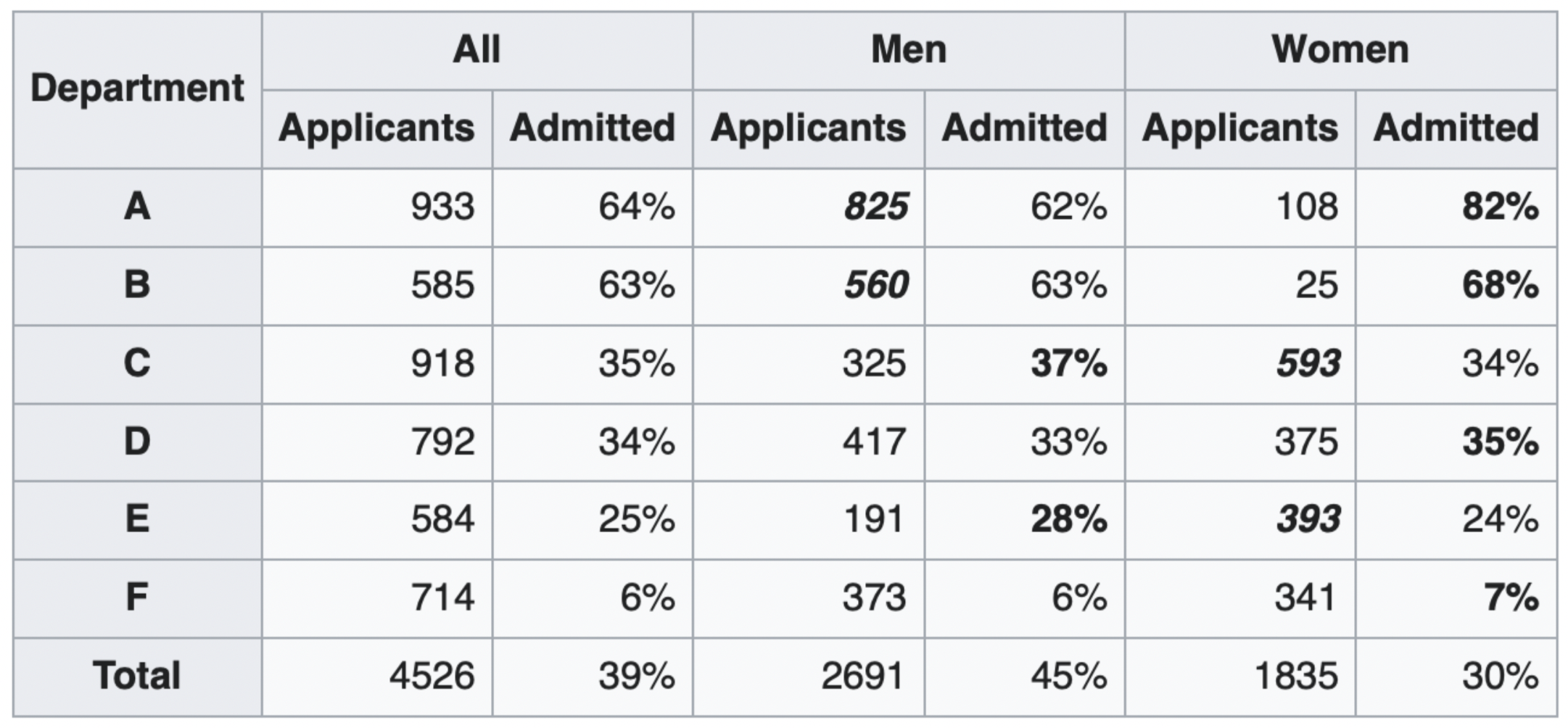
show_paradox_slides()
What happened?
The overall acceptance rate for women (30%) was lower than it was for men (45%).
However, most departments (A, B, D, F) had a higher acceptance rate for women.
Department A had a 62% acceptance rate for men and an 82% acceptance rate for women!
- 31% of men applied to Department A.
- 6% of women applied to Department A.
Department F had a 6% acceptance rate for men and a 7% acceptance rate for women!
- 14% of men applied to Department F.
- 19% of women applied to Department F.
Conclusion: Women tended to apply to departments with a lower acceptance rate; the data don't support the hypothesis that there was major gender discrimination against women.
Example: Restaurant reviews and phone types
You are deciding whether to eat at Dirty Birds or The Loft.
Suppose Yelp shows ratings aggregated by phone type (Android vs. iPhone).
| Phone Type | Stars for Dirty Birds | Stars for The Loft |
|---|---|---|
| Android | 4.24 | 4.0 |
| iPhone | 2.99 | 2.79 |
| All | 3.32 | 3.37 |
Question: Should you choose Dirty Birds or The Loft?
Answer: The type of phone you use likely has nothing to do with your taste in food – pick the restaurant that is rated higher overall.
Rule of thumb 👍
Let $(X, Y)$ be a pair of variables of interest. Simpson's paradox occurs when the association between $X$ and $Y$ reverses when we condition on $Z$, a third variable.
If $Z$ has a causal connection to both $X$ and $Y$, we should condition on $Z$ and use deaggregated data.
If not, we shouldn't condition on $Z$ and use the aggregated data instead.
Berkeley gender discrimination: $X$ is gender, $Y$ is acceptance rate. $Z$ is the department.
- $Z$ has a plausible causal effect on both $X$ and $Y$, so we should condition on $Z$.
Yelp ratings: $X$ is the restaurant, $Y$ is the average stars. $Z$ is the phone type.
- $Z$ doesn't plausibly cause $X$ to change, so we should not condition on $Z$.
Takeaways
Be skeptical of...
- Aggregate statistics.
- People misusing statistics to "prove" that discrimination doesn't exist.
- Drawing conclusions from individual publications ($p$-hacking, publication bias, narrow focus, etc.).
- Everything!
We need to apply domain knowledge and human judgement calls to decide what to do when Simpson's paradox is present.
Really?
To handle Simpson's paradox with rigor, we need some ideas from causal inference which we don't have time to cover in DSC 80. This video has a good example of how to approach Simpson's paradox using a minimal amount of causal inference, if you're curious (not required for DSC 80).
IFrame('https://www.youtube-nocookie.com/embed/zeuW1Z2EtLs?si=l2Dl7P-5RCq3ODpo',
width=800, height=450)
Further reading
- Gender Bias in Admission Statistics?
- Contains a great visualization, but seems to be paywalled now.
- What is Simpson's Paradox?
- Understanding Simpson's Paradox
- Requires more statistics background, but gives a rigorous understanding of when to use aggregated vs. unaggregated data.
Merging
Example: Name categories
The New York Times article from Lecture 1 claims that certain categories of names are becoming more popular. For example:
Forbidden names like Lucifer, Lilith, Kali, and Danger.
Evangelical names like Amen, Savior, Canaan, and Creed.
Mythological names.
It also claims that baby boomer names are becoming less popular.
Let's see if we can verify these claims using data!
Loading in the data
Our first DataFrame, baby, is the same as we saw in Lecture 1. It has one row for every combination of 'Name', 'Sex', and 'Year'.
baby_path = Path('data') / 'baby.csv'
baby = pd.read_csv(baby_path)
baby
| Name | Sex | Count | Year | |
|---|---|---|---|---|
| 0 | Liam | M | 20456 | 2022 |
| 1 | Noah | M | 18621 | 2022 |
| 2 | Olivia | F | 16573 | 2022 |
| ... | ... | ... | ... | ... |
| 2085155 | Wright | M | 5 | 1880 |
| 2085156 | York | M | 5 | 1880 |
| 2085157 | Zachariah | M | 5 | 1880 |
2085158 rows × 4 columns
Our second DataFrame, nyt, contains the New York Times' categorization of each of several names, based on the aforementioned article.
nyt_path = Path('data') / 'nyt_names.csv'
nyt = pd.read_csv(nyt_path)
nyt
| nyt_name | category | |
|---|---|---|
| 0 | Lucifer | forbidden |
| 1 | Lilith | forbidden |
| 2 | Danger | forbidden |
| ... | ... | ... |
| 20 | Venus | celestial |
| 21 | Celestia | celestial |
| 22 | Skye | celestial |
23 rows × 2 columns
Issue: To find the number of babies born with (for example) forbidden names each year, we need to combine information from both baby and nyt.
Merging
- We want to link rows from
babyandnyttogether whenever the names match up. - This is a merge (
pandasterm), i.e. a join (SQL term). - A merge is appropriate when we have two sources of information about the same individuals that is linked by a common column(s).
- The common column(s) are called the join key.
Example merge
Let's demonstrate on a small subset of baby and nyt.
nyt_small = nyt.iloc[[11, 12, 14]].reset_index(drop=True)
names_to_keep = ['Julius', 'Karen', 'Noah']
baby_small = (baby
.query("Year == 2020 and Name in @names_to_keep")
.reset_index(drop=True)
)
dfs_side_by_side(baby_small, nyt_small)
| Name | Sex | Count | Year | |
|---|---|---|---|---|
| 0 | Noah | M | 18407 | 2020 |
| 1 | Julius | M | 966 | 2020 |
| 2 | Karen | F | 330 | 2020 |
| 3 | Noah | F | 306 | 2020 |
| 4 | Karen | M | 6 | 2020 |
| nyt_name | category | |
|---|---|---|
| 0 | Karen | boomer |
| 1 | Julius | mythology |
| 2 | Freya | mythology |
%%pt
baby_small.merge(nyt_small, left_on='Name', right_on='nyt_name')
The merge method
The
mergeDataFrame method joins two DataFrames by columns or indexes.- As mentioned before, "merge" is just the
pandasword for "join."
- As mentioned before, "merge" is just the
When using the
mergemethod, the DataFrame beforemergeis the "left" DataFrame, and the DataFrame passed intomergeis the "right" DataFrame.- In
baby_small.merge(nyt_small),baby_smallis considered the "left" DataFrame andnyt_smallis the "right" DataFrame; the columns from the left DataFrame appear to the left of the columns from right DataFrame.
- In
By default:
- If join keys are not specified, all shared columns between the two DataFrames are used.
- The "type" of join performed is an inner join. This is the only type of join you saw in DSC 10, but there are more, as we'll now see!
Join types: inner joins
%%pt
baby_small.merge(nyt_small, left_on='Name', right_on='nyt_name')
- Note that
'Noah'and'Freya'do not appear in the merged DataFrame. - This is because there is:
- no
'Noah'in the right DataFrame (nyt_small), and - no
'Freya'in the left DataFrame (baby_small).
- no
- The default type of join that
mergeperforms is an inner join, which keeps the intersection of the join keys.

Different join types
We can change the type of join performed by changing the how argument in merge. Let's experiment!
%%pt
# Note the NaNs!
baby_small.merge(nyt_small, left_on='Name', right_on='nyt_name', how='left')
%%pt
baby_small.merge(nyt_small, left_on='Name', right_on='nyt_name', how='right')
%%pt
baby_small.merge(nyt_small, left_on='Name', right_on='nyt_name', how='outer')
Different join types handle mismatches differently
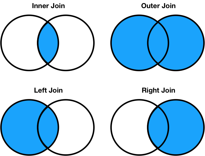
There are four types of joins.
- Inner: keep only matching keys (intersection).
- Outer: keep all keys in both DataFrames (union).
- Left: keep all keys in the left DataFrame, whether or not they are in the right DataFrame.
- Right: keep all keys in the right DataFrame, whether or not they are in the left DataFrame.
- Note that
a.merge(b, how='left')contains the same information asb.merge(a, how='right'), just in a different order.
- Note that
Notes on the merge method
mergeis flexible – you can merge using a combination of columns, or the index of the DataFrame.- If the two DataFrames have the same column names,
pandaswill add_xand_yto the duplicated column names to avoid having columns with the same name (change these thesuffixesargument). - There is, in fact, a
joinmethod, but it's actually a wrapper aroundmergewith fewer options. - As always, the documentation is your friend!
Lots of pandas operations do an implicit outer join!
pandaswill almost always try to match up index values using an outer join.- It won't tell you that it's doing an outer join, it'll just throw
NaNs in your result!
df1 = pd.DataFrame({'a': [1, 2, 3]}, index=['hello', 'dsc80', 'students'])
df2 = pd.DataFrame({'b': [10, 20, 30]}, index=['dsc80', 'is', 'awesome'])
dfs_side_by_side(df1, df2)
| a | |
|---|---|
| hello | 1 |
| dsc80 | 2 |
| students | 3 |
| b | |
|---|---|
| dsc80 | 10 |
| is | 20 |
| awesome | 30 |
df1['a'] + df2['b']
awesome NaN dsc80 12.0 hello NaN is NaN students NaN dtype: float64
Many-to-one & many-to-many joins
One-to-one joins
- So far in this lecture, the joins we have worked with are called one-to-one joins.
- Neither the left DataFrame (
baby_small) nor the right DataFrame (nyt_small) contained any duplicates in the join key. - What if there are duplicated join keys, in one or both of the DataFrames we are merging?
# Run this cell to set up the next example.
profs = pd.DataFrame(
[['Sam', 'UCB', 5],
['Sam', 'UCSD', 5],
['Janine', 'UCSD', 8],
['Marina', 'UIC', 7],
['Justin', 'OSU', 5],
['Soohyun', 'UCSD', 2],
['Suraj', 'UCB', 2]],
columns=['Name', 'School', 'Years']
)
schools = pd.DataFrame({
'Abr': ['UCSD', 'UCLA', 'UCB', 'UIC'],
'Full': ['University of California San Diego', 'University of California, Los Angeles', 'University of California, Berkeley', 'University of Illinois Chicago']
})
programs = pd.DataFrame({
'uni': ['UCSD', 'UCSD', 'UCSD', 'UCB', 'OSU', 'OSU'],
'dept': ['Math', 'HDSI', 'COGS', 'CS', 'Math', 'CS'],
'grad_students': [205, 54, 281, 439, 304, 193]
})
Many-to-one joins
- Many-to-one joins are joins where one of the DataFrames contains duplicate values in the join key.
- The resulting DataFrame will preserve those duplicate entries as appropriate.
dfs_side_by_side(profs, schools)
| Name | School | Years | |
|---|---|---|---|
| 0 | Sam | UCB | 5 |
| 1 | Sam | UCSD | 5 |
| 2 | Janine | UCSD | 8 |
| 3 | Marina | UIC | 7 |
| 4 | Justin | OSU | 5 |
| 5 | Soohyun | UCSD | 2 |
| 6 | Suraj | UCB | 2 |
| Abr | Full | |
|---|---|---|
| 0 | UCSD | University of California San Diego |
| 1 | UCLA | University of California, Los Angeles |
| 2 | UCB | University of California, Berkeley |
| 3 | UIC | University of Illinois Chicago |
Note that when merging profs and schools, the information from schools is duplicated.
'University of California, San Diego'appears three times.'University of California, Berkeley'appears twice.
%%pt
profs.merge(schools, left_on='School', right_on='Abr', how='left')
Many-to-many joins
Many-to-many joins are joins where both DataFrames have duplicate values in the join key.
dfs_side_by_side(profs, programs)
| Name | School | Years | |
|---|---|---|---|
| 0 | Sam | UCB | 5 |
| 1 | Sam | UCSD | 5 |
| 2 | Janine | UCSD | 8 |
| 3 | Marina | UIC | 7 |
| 4 | Justin | OSU | 5 |
| 5 | Soohyun | UCSD | 2 |
| 6 | Suraj | UCB | 2 |
| uni | dept | grad_students | |
|---|---|---|---|
| 0 | UCSD | Math | 205 |
| 1 | UCSD | HDSI | 54 |
| 2 | UCSD | COGS | 281 |
| 3 | UCB | CS | 439 |
| 4 | OSU | Math | 304 |
| 5 | OSU | CS | 193 |
Before running the following cell, try predicting the number of rows in the output.
%%pt
profs.merge(programs, left_on='School', right_on='uni', how='inner')
mergestitched together every UCSD row inprofswith every UCSD row inprograms.- Since there were 3 UCSD rows in
profsand 3 inprograms, there are $3 \cdot 3 = 9$ UCSD rows in the output. The same applies for all other schools.
Question 🤔 (Answer at dsc80.com/q)
Code: lec04-merge
Fill in the blank so that the last statement evaluates to True.
df = profs.merge(programs, left_on='School', right_on='uni')
df.shape[0] == (____).sum()
Don't use merge (or join) in your solution!
dfs_side_by_side(profs, programs)
# Your code goes here.
Returning back to our original question
Let's find the popularity of baby name categories over time. To start, we'll define a DataFrame that has one row for every combination of 'category' and 'Year'.
cate_counts = (
baby
.merge(nyt, left_on='Name', right_on='nyt_name')
.groupby(['category', 'Year'])
['Count']
.sum()
.reset_index()
)
cate_counts
| category | Year | Count | |
|---|---|---|---|
| 0 | boomer | 1880 | 292 |
| 1 | boomer | 1881 | 298 |
| 2 | boomer | 1882 | 326 |
| ... | ... | ... | ... |
| 659 | mythology | 2020 | 3516 |
| 660 | mythology | 2021 | 3895 |
| 661 | mythology | 2022 | 4049 |
662 rows × 3 columns
# We'll talk about plotting code soon!
import plotly.express as px
fig = px.line(cate_counts, x='Year', y='Count',
facet_col='category', facet_col_wrap=3,
facet_row_spacing=0.15,
width=600, height=400)
fig.update_yaxes(matches=None, showticklabels=False)
Questions? 🤔
%%timeit
baby['Name'].apply(number_of_vowels)
%%timeit
res = []
for name in baby['Name']:
res.append(number_of_vowels(name))
Internally, apply actually just runs a for-loop!
So, when possible – say, when applying arithmetic operations – we should work on Series objects directly and avoid apply!
Other data representations
Representations of tabular data
In DSC 80, we work with DataFrames in
pandas.- When we say
pandasDataFrame, we're talking about thepandasAPI for its DataFrame objects.- API stands for "application programming interface." We'll learn about these more soon.
- When we say "DataFrame", we're referring to a general way to represent data (rows and columns, with labels for both rows and columns).
- When we say
There many other ways to work with data tables!
- Examples: R data frames, SQL databases, spreadsheets, or even matrices from linear algebra.
- When you learn SQL in DSC 100, you'll find many similaries (e.g. slicing columns, filtering rows, grouping, joining, etc.).
- Relational algebra captures common data operations between many data table systems.
Why use DataFrames over something else?
DataFrames vs. spreadsheets
- DataFrames give us a data lineage: the code records down data changes. Not so in spreadsheets!
- Using a general-purpose programming language gives us the ability to handle much larger datasets, and we can use distributed computing systems to handle massive datasets.
DataFrames vs. matrices
\begin{split} \begin{aligned} \mathbf{X} = \begin{bmatrix} 1 & 0 \\ 0 & 4 \\ 0 & 0 \\ \end{bmatrix} \end{aligned} \end{split}
- Matrices are mathematical objects. They only hold numbers, but have many useful properties (which you've learned about in your linear algebra class, Math 18).
- Often, we process data from a DataFrame into matrix format for machine learning models. You saw this a bit in DSC 40A, and we'll see this more in DSC 80 in a few weeks.
DataFrames vs. relations
- Relations are the data representation for relational database systems (e.g. MySQL, PostgreSQL, etc.).
- You'll learn all about these in DSC 100.
- Database systems are much better than DataFrames at storing many large data tables and handling concurrency (many people reading and writing data at the same time).
- Common workflow: load a subset of data in from a database system into
pandas, then make a plot. - Or: load and clean data in
pandas, then store it in a database system for others to use.
Summary
- There is no "formula" to automatically resolve Simpson's paradox! Domain knowledge is important.
- We've covered most of the primary DataFrame operations: subsetting, aggregating, joining, and transforming.
Next time
Data cleaning: applying what we've already learned to real-world, messy data!