from dsc80_utils import *
Agenda 📆
- Dataset overview.
- Introduction to
plotly. - Exploratory data analysis and feature types.
- Data cleaning.
- Data quality checks.
- Missing values.
- Transformations and timestamps.
- Modifying structure.
- Investigating student-submitted questions!
Dataset overview
San Diego food safety
From this article (archive link):
In the last three years, one third of San Diego County restaurants have had at least one major food safety violation.
99% Of San Diego Restaurants Earn ‘A' Grades, Bringing Usefulness of System Into Question
From this article (archive link):
Food held at unsafe temperatures. Employees not washing their hands. Dirty countertops. Vermin in the kitchen. An expired restaurant permit.
Restaurant inspectors for San Diego County found these violations during a routine health inspection of a diner in La Mesa in November 2016. Despite the violations, the restaurant was awarded a score of 90 out of 100, the lowest possible score to achieve an ‘A’ grade.
The data
- We downloaded the data about the 1000 restaurants closest to UCSD from here.
- We had to download the data as JSON files, then process it into DataFrames. You'll learn how to do this soon!
- Until now, you've (largely) been presented with CSV files that
pd.read_csvcould load without any issues. - But there are many different formats and possible issues when loading data in from files.
- See Chapter 8 of Learning DS for more.
- Until now, you've (largely) been presented with CSV files that
rest_path = Path('data') / 'restaurants.csv'
insp_path = Path('data') / 'inspections.csv'
viol_path = Path('data') / 'violations.csv'
rest = pd.read_csv(rest_path)
insp = pd.read_csv(insp_path)
viol = pd.read_csv(viol_path)
Question 🤔 (Answer at dsc80.com/q)
Code: lec05-dfs
The first article said that one third of restaurants had at least one major safety violation.
Which DataFrames and columns seem most useful to verify this?
rest.head(2)
| business_id | name | business_type | address | ... | lat | long | opened_date | distance | |
|---|---|---|---|---|---|---|---|---|---|
| 0 | 211898487641 | MOBIL MART LA JOLLA VILLAGE | Pre-Packaged Retail Market | 3233 LA JOLLA VILLAGE DR, LA JOLLA, CA 92037 | ... | 32.87 | -117.23 | 2002-05-05 | 0.62 |
| 1 | 211930769329 | CAFE 477 | Low Risk Food Facility | 8950 VILLA LA JOLLA DR, SUITE# B123, LA JOLLA,... | ... | 32.87 | -117.24 | 2023-07-24 | 0.64 |
2 rows × 12 columns
rest.columns
Index(['business_id', 'name', 'business_type', 'address', 'city', 'zip',
       'phone', 'status', 'lat', 'long', 'opened_date', 'distance'],
      dtype='object')
insp.head(2)
| custom_id | business_id | inspection_id | description | ... | completed_date | status | link | status_link | |
|---|---|---|---|---|---|---|---|---|---|
| 0 | DEH2002-FFPN-310012 | 211898487641 | 6886133 | NaN | ... | 2023-02-16 | Complete | http://www.sandiegocounty.gov/deh/fhd/ffis/ins... | http://www.sandiegocounty.gov/deh/fhd/ffis/ins... |
| 1 | DEH2002-FFPN-310012 | 211898487641 | 6631228 | NaN | ... | 2022-01-03 | Complete | http://www.sandiegocounty.gov/deh/fhd/ffis/ins... | http://www.sandiegocounty.gov/deh/fhd/ffis/ins... |
2 rows × 11 columns
insp.columns
Index(['custom_id', 'business_id', 'inspection_id', 'description', 'type',
       'score', 'grade', 'completed_date', 'status', 'link', 'status_link'],
      dtype='object')
viol.head(2)
| inspection_id | violation | major_violation | status | violation_text | correction_type_link | violation_accela | link | |
|---|---|---|---|---|---|---|---|---|
| 0 | 6886133 | Hot and Cold Water | Y | Out of Compliance - Major | Hot and Cold Water | http://www.sandiegocounty.gov/deh/fhd/ffis/vio... | 21. Hot & cold water available | http://www.sandiegocounty.gov/deh/fhd/ffis/vio... |
| 1 | 6631228 | Hot and Cold Water | N | Out of Compliance - Minor | Hot and Cold Water | http://www.sandiegocounty.gov/deh/fhd/ffis/vio... | 21. Hot & cold water available | http://www.sandiegocounty.gov/deh/fhd/ffis/vio... |
viol.columns
Index(['inspection_id', 'violation', 'major_violation', 'status',
       'violation_text', 'correction_type_link', 'violation_accela', 'link'],
      dtype='object')
Introduction to plotly
plotly
- We've used
plotlyin lecture briefly, and you even have to use it in Project 1 Question 13, but we haven't yet discussed it formally.
- It's a visualization library that enables interactive visualizations.

Using plotly
There are a few ways we can use plotly:
- Using the
plotly.expresssyntax.plotlyis very flexible, but it can be verbose;plotly.expressallows us to make plots quickly.- See the documentation here – it's very rich (there are good examples for almost everything).
- By setting
pandasplotting backend to'plotly'(by default, it's'matplotlib') and using the DataFrameplotmethod.- The DataFrame
plotmethod is how you created plots in DSC 10!
- The DataFrame
For now, we'll use plotly.express syntax; we've imported it in the dsc80_utils.py file that we import at the top of each lecture notebook.
Initial plots
First, let's look at the distribution of inspection 'score's:
#insp['score']
fig = px.histogram(insp['score'])
fig
How about the distribution of average inspection 'score' per 'grade'?
scores = (
    insp[['grade', 'score']]
    .dropna()
    .groupby('grade')
    .mean()
    .reset_index()
)
#scores
# x= and y= are columns of scores. Convenient!
px.bar(scores, x='grade', y='score')
# Same as the above!
scores.plot(kind='bar', x='grade', y='score')
Exploratory data analysis and feature types

Exploratory data analysis (EDA)
Historically, data analysis was dominated by formal statistics, including tools like confidence intervals, hypothesis tests, and statistical modeling.
In 1977, John Tukey defined the term exploratory data analysis, which described a philosophy for proceeding about data analysis:
Exploratory data analysis is actively incisive, rather than passively descriptive, with real emphasis on the discovery of the unexpected.
- Practically, EDA involves, among other things, computing summary statistics and drawing plots to understand the nature of the data at hand.
The greatest gains from data come from surprises… The unexpected is best brought to our attention by pictures.
Different feature types
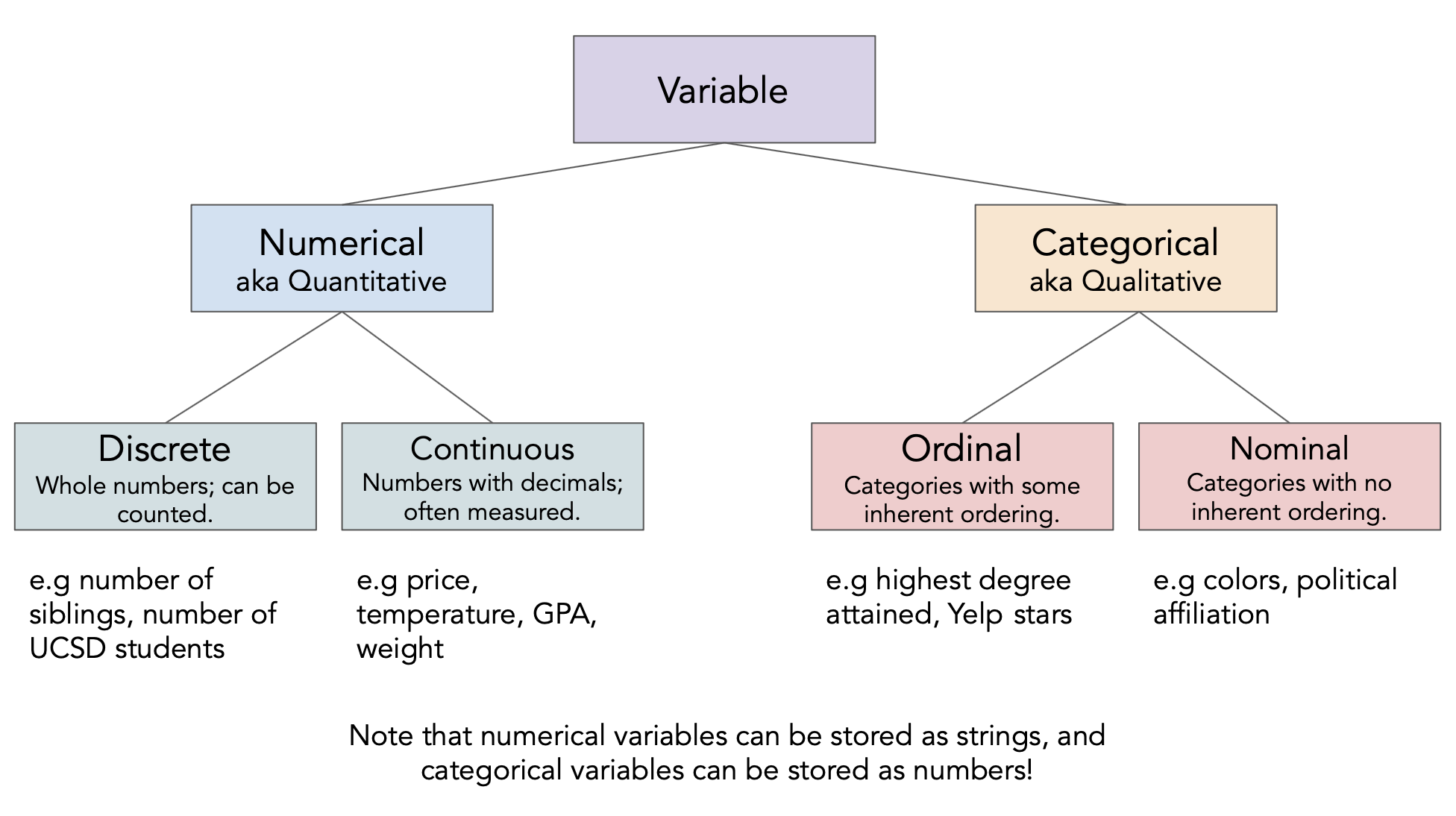
Question 🤔 (Answer at dsc80.com/q)
Code: lec05-types
Determine the feature type of each of the following variables.
insp['score']insp['grade']viol['violation_accela']viol['major_violation']rest['business_id']rest['opened_date']
...
Ellipsis
Feature types vs. data types
The data type
pandasuses is not the same as the "data type" we talked about just now!- There's a difference between feature type and computational data type.
Take care when the two don't match up very well!
# pandas stores these as ints, but they're actually nominal.
rest['business_id']
0      211898487641
1      211930769329
2      211909057778
           ...
997    211899338714
998    211942150255
999    211925713322
Name: business_id, Length: 1000, dtype: int64
# pandas stores these as strings, but they're actually numeric.
rest['opened_date']
0      2002-05-05
1      2023-07-24
2      2019-01-22
          ...
997    2002-05-05
998    2016-11-03
999    2022-11-03
Name: opened_date, Length: 1000, dtype: object
Data cleaning
Four pillars of data cleaning
When loading in a dataset, to clean the data – that is, to prepare it for further analysis – we will:
Perform data quality checks.
Identify and handle missing values.
Perform transformations, including converting time series data to timestamps.
Modify structure as necessary.
Data cleaning: Data quality checks
Data quality checks
We often start an analysis by checking the quality of the data.
- Scope: Do the data match your understanding of the population?
- Measurements and values: Are the values reasonable?
- Relationships: Are related features in agreement?
- Analysis: Which features might be useful in a future analysis?
Scope
Do the data match your understanding of the population?
We were told that we're only looking at the 1000 restaurants closest to UCSD, so the restaurants in rest should agree with that.
rest.sample(5)
| business_id | name | business_type | address | ... | lat | long | opened_date | distance | |
|---|---|---|---|---|---|---|---|---|---|
| 869 | 211912304517 | SWEET MAHINA | Class B Cottage Food Operation | 4551 MT LA PLATTA PL, SAN DIEGO, CA 92117-3045 | ... | 32.83 | -117.19 | 2021-08-31 | 4.47 |
| 935 | 211906499771 | THE GOLF BAR | Restaurant Food Facility | 5583 CLAIREMONT MESA BLVD, SAN DIEGO, CA 92117 | ... | 32.83 | -117.17 | 2019-10-11 | 4.84 |
| 187 | 211984552427 | LEMONADE | Restaurant Food Facility | 4545 LA JOLLA VILLAGE DR, SUITE# D-35, SAN DIE... | ... | 32.87 | -117.21 | 2014-12-12 | 1.51 |
| 902 | 211944527313 | DAVANTI ENOTECA | Restaurant Food Facility | 12955 EL CAMINO REAL, SUITE# G-3, SAN DIEGO, C... | ... | 32.95 | -117.24 | 2020-02-24 | 4.68 |
| 640 | 211903875703 | MAGDA'S BAKERY | Class A Cottage Food Operation | 6505 MUIRLANDS DR, LA JOLLA, CA 92037-6350 | ... | 32.83 | -117.26 | 2020-09-16 | 3.76 |
5 rows × 12 columns
Measurements and values
Are the values reasonable?
Do the values in the 'grade' column match what we'd expect grades to look like?
insp['grade'].value_counts()
grade
A    2978
B      11
Name: count, dtype: int64
What kinds of information does the insp DataFrame hold?
insp.info()
<class 'pandas.core.frame.DataFrame'>
RangeIndex: 5179 entries, 0 to 5178
Data columns (total 11 columns):
 #   Column          Non-Null Count  Dtype
---  ------          --------------  -----
 0   custom_id       5179 non-null   object
 1   business_id     5179 non-null   int64
 2   inspection_id   5179 non-null   int64
 3   description     0 non-null      float64
 4   type            5179 non-null   object
 5   score           5179 non-null   int64
 6   grade           2989 non-null   object
 7   completed_date  5179 non-null   object
 8   status          5179 non-null   object
 9   link            5179 non-null   object
 10  status_link     5179 non-null   object
dtypes: float64(1), int64(3), object(7)
memory usage: 445.2+ KB
What's going on in the 'address' column of rest?
# Are there multiple restaurants with the same address?
rest['address'].value_counts()
address
5300 GRAND DEL MAR CT, SAN DIEGO, CA 92130       9
8657 VILLA LA JOLLA DR, LA JOLLA, CA 92037       8
4545 LA JOLLA VILLAGE DR, SAN DIEGO, CA 92122    8
                                                ..
3963 GOVERNOR DR, SAN DIEGO, CA 92122            1
4041 GOVERNOR DR, SAN DIEGO, CA 92122-2520       1
2672 DEL MAR HEIGHTS RD, DEL MAR, CA 92014       1
Name: count, Length: 863, dtype: int64
# Keeps all rows with duplicate addresses.
(
    rest
    .groupby('address')
    .filter(lambda df: df.shape[0] >= 2)
    .sort_values('address')
)
| business_id | name | business_type | address | ... | lat | long | opened_date | distance | |
|---|---|---|---|---|---|---|---|---|---|
| 406 | 211899308875 | NASEEMS BAKERY & KABOB | Restaurant Food Facility | 10066 PACIFIC HEIGHTS BLVD, SAN DIEGO, CA 92121 | ... | 32.90 | -117.19 | 2012-04-17 | 2.77 |
| 402 | 211898699154 | HANAYA SUSHI CAFE | Restaurant Food Facility | 10066 PACIFIC HEIGHTS BLVD, SAN DIEGO, CA 92121 | ... | 32.90 | -117.19 | 2011-03-22 | 2.77 |
| 401 | 211899558107 | ARMANDOS MEXICAN FOOD | Restaurant Food Facility | 10066 PACIFIC HEIGHTS BLVD, SAN DIEGO, CA 92121 | ... | 32.90 | -117.19 | 2005-06-28 | 2.77 |
| ... | ... | ... | ... | ... | ... | ... | ... | ... | ... |
| 575 | 211972411855 | TARA HEATHER CAKE DESIGN | Caterer | 9932 MESA RIM RD, SUITE# A, SAN DIEGO, CA 9212... | ... | 32.90 | -117.18 | 2014-04-24 | 3.51 |
| 344 | 211990537315 | COMPASS GROUP FEDEX EXPRESS OLSON | Pre-Packaged Retail Market | 9999 OLSON DR, SAN DIEGO, CA 92121-2837 | ... | 32.89 | -117.20 | 2022-10-19 | 2.27 |
| 343 | 211976587262 | CANTEEN - FED EX OLSON | Pre-Packaged Retail Market | 9999 OLSON DR, SAN DIEGO, CA 92121-2837 | ... | 32.89 | -117.20 | 2020-07-31 | 2.27 |
213 rows × 12 columns
# Does the same thing as above!
(
    rest[rest.duplicated(subset=['address'], keep=False)]
    .sort_values('address')
)
| business_id | name | business_type | address | ... | lat | long | opened_date | distance | |
|---|---|---|---|---|---|---|---|---|---|
| 406 | 211899308875 | NASEEMS BAKERY & KABOB | Restaurant Food Facility | 10066 PACIFIC HEIGHTS BLVD, SAN DIEGO, CA 92121 | ... | 32.90 | -117.19 | 2012-04-17 | 2.77 |
| 402 | 211898699154 | HANAYA SUSHI CAFE | Restaurant Food Facility | 10066 PACIFIC HEIGHTS BLVD, SAN DIEGO, CA 92121 | ... | 32.90 | -117.19 | 2011-03-22 | 2.77 |
| 401 | 211899558107 | ARMANDOS MEXICAN FOOD | Restaurant Food Facility | 10066 PACIFIC HEIGHTS BLVD, SAN DIEGO, CA 92121 | ... | 32.90 | -117.19 | 2005-06-28 | 2.77 |
| ... | ... | ... | ... | ... | ... | ... | ... | ... | ... |
| 575 | 211972411855 | TARA HEATHER CAKE DESIGN | Caterer | 9932 MESA RIM RD, SUITE# A, SAN DIEGO, CA 9212... | ... | 32.90 | -117.18 | 2014-04-24 | 3.51 |
| 344 | 211990537315 | COMPASS GROUP FEDEX EXPRESS OLSON | Pre-Packaged Retail Market | 9999 OLSON DR, SAN DIEGO, CA 92121-2837 | ... | 32.89 | -117.20 | 2022-10-19 | 2.27 |
| 343 | 211976587262 | CANTEEN - FED EX OLSON | Pre-Packaged Retail Market | 9999 OLSON DR, SAN DIEGO, CA 92121-2837 | ... | 32.89 | -117.20 | 2020-07-31 | 2.27 |
213 rows × 12 columns
Relationships
Are related features in agreement?
Do the 'address'es and 'zip' codes in rest match?
rest[['address', 'zip']]
| address | zip | |
|---|---|---|
| 0 | 3233 LA JOLLA VILLAGE DR, LA JOLLA, CA 92037 | 92037 |
| 1 | 8950 VILLA LA JOLLA DR, SUITE# B123, LA JOLLA,... | 92037-1704 |
| 2 | 6902 LA JOLLA BLVD, LA JOLLA, CA 92037 | 92037 |
| ... | ... | ... |
| 997 | 1234 TOURMALINE ST, SAN DIEGO, CA 92109-1856 | 92109-1856 |
| 998 | 12925 EL CAMINO REAL, SUITE# AA4, SAN DIEGO, C... | 92130 |
| 999 | 2672 DEL MAR HEIGHTS RD, DEL MAR, CA 92014 | 92014 |
1000 rows × 2 columns
What about the 'score's and 'grade's in insp?
insp[['score', 'grade']]
| score | grade | |
|---|---|---|
| 0 | 96 | NaN |
| 1 | 98 | NaN |
| 2 | 98 | NaN |
| ... | ... | ... |
| 5176 | 0 | NaN |
| 5177 | 0 | NaN |
| 5178 | 90 | A |
5179 rows × 2 columns
Analysis
Which features might be useful in a future analysis?
We're most interested in:
- These columns in the
restDataFrame:'business_id','name','address','zip', and'opened_date'. - These columns in the
inspDataFrame:'business_id','inspection_id','score','grade','completed_date', and'status'. - These columns in the
violDataFrame:'inspection_id','violation','major_violation','violation_text', and'violation_accela'.
- These columns in the
Also, let's rename a few columns to make them easier to work with.
💡 Pro-Tip: Using pipe
When we manipulate DataFrames, it's best to define individual functions for each step, then use the pipe method to chain them all together.
The pipe DataFrame method takes in a function, which itself takes in a DataFrame and returns a DataFrame.
- In practice, we would add functions one by one to the top of a notebook, then
pipethem all. - For today, will keep re-running
pipeto show data cleaning process.
def subset_rest(rest):
    return rest[['business_id', 'name', 'address', 'zip', 'opened_date']]

rest = (
    pd.read_csv(rest_path)
    .pipe(subset_rest)
)
rest
| business_id | name | address | zip | opened_date | |
|---|---|---|---|---|---|
| 0 | 211898487641 | MOBIL MART LA JOLLA VILLAGE | 3233 LA JOLLA VILLAGE DR, LA JOLLA, CA 92037 | 92037 | 2002-05-05 |
| 1 | 211930769329 | CAFE 477 | 8950 VILLA LA JOLLA DR, SUITE# B123, LA JOLLA,... | 92037-1704 | 2023-07-24 |
| 2 | 211909057778 | VALLEY FARM MARKET | 6902 LA JOLLA BLVD, LA JOLLA, CA 92037 | 92037 | 2019-01-22 |
| ... | ... | ... | ... | ... | ... |
| 997 | 211899338714 | PACIFIC BEACH ELEMENTARY | 1234 TOURMALINE ST, SAN DIEGO, CA 92109-1856 | 92109-1856 | 2002-05-05 |
| 998 | 211942150255 | POKEWAN DEL MAR | 12925 EL CAMINO REAL, SUITE# AA4, SAN DIEGO, C... | 92130 | 2016-11-03 |
| 999 | 211925713322 | SAFFRONO LOUNGE RESTAURANT | 2672 DEL MAR HEIGHTS RD, DEL MAR, CA 92014 | 92014 | 2022-11-03 |
1000 rows × 5 columns
# Same as the above – but the above makes it easier to chain more .pipe calls afterwards.
subset_rest(pd.read_csv(rest_path))
| business_id | name | address | zip | opened_date | |
|---|---|---|---|---|---|
| 0 | 211898487641 | MOBIL MART LA JOLLA VILLAGE | 3233 LA JOLLA VILLAGE DR, LA JOLLA, CA 92037 | 92037 | 2002-05-05 |
| 1 | 211930769329 | CAFE 477 | 8950 VILLA LA JOLLA DR, SUITE# B123, LA JOLLA,... | 92037-1704 | 2023-07-24 |
| 2 | 211909057778 | VALLEY FARM MARKET | 6902 LA JOLLA BLVD, LA JOLLA, CA 92037 | 92037 | 2019-01-22 |
| ... | ... | ... | ... | ... | ... |
| 997 | 211899338714 | PACIFIC BEACH ELEMENTARY | 1234 TOURMALINE ST, SAN DIEGO, CA 92109-1856 | 92109-1856 | 2002-05-05 |
| 998 | 211942150255 | POKEWAN DEL MAR | 12925 EL CAMINO REAL, SUITE# AA4, SAN DIEGO, C... | 92130 | 2016-11-03 |
| 999 | 211925713322 | SAFFRONO LOUNGE RESTAURANT | 2672 DEL MAR HEIGHTS RD, DEL MAR, CA 92014 | 92014 | 2022-11-03 |
1000 rows × 5 columns
Let's use pipe to keep (and rename) the subset of the columns we care about in the other two DataFrames as well.
def subset_insp(insp):
    return (
        insp[['business_id', 'inspection_id', 'score', 'grade', 'completed_date', 'status']]
        .rename(columns={'completed_date': 'date'})
    )

insp = (
    pd.read_csv(insp_path)
    .pipe(subset_insp)
)
def subset_viol(viol):
    return (
        viol[['inspection_id', 'violation', 'major_violation', 'violation_accela']]
        .rename(columns={'violation': 'kind',
                         'major_violation': 'is_major',
                         'violation_accela': 'violation'})
    )

viol = (
    pd.read_csv(viol_path)
    .pipe(subset_viol)
)
Combining the restaurant data
Let's join all three DataFrames together so that we have all the data in a single DataFrame.
def merge_all_restaurant_data():
    return (
        rest
        .merge(insp, on='business_id', how='left')
        .merge(viol, on='inspection_id', how='left')
    )

df = merge_all_restaurant_data()
df
| business_id | name | address | zip | ... | status | kind | is_major | violation | |
|---|---|---|---|---|---|---|---|---|---|
| 0 | 211898487641 | MOBIL MART LA JOLLA VILLAGE | 3233 LA JOLLA VILLAGE DR, LA JOLLA, CA 92037 | 92037 | ... | Complete | Hot and Cold Water | Y | 21. Hot & cold water available |
| 1 | 211898487641 | MOBIL MART LA JOLLA VILLAGE | 3233 LA JOLLA VILLAGE DR, LA JOLLA, CA 92037 | 92037 | ... | Complete | Hot and Cold Water | N | 21. Hot & cold water available |
| 2 | 211898487641 | MOBIL MART LA JOLLA VILLAGE | 3233 LA JOLLA VILLAGE DR, LA JOLLA, CA 92037 | 92037 | ... | Complete | Holding Temperatures | N | 7. Proper hot & cold holding temperatures |
| ... | ... | ... | ... | ... | ... | ... | ... | ... | ... |
| 8728 | 211925713322 | SAFFRONO LOUNGE RESTAURANT | 2672 DEL MAR HEIGHTS RD, DEL MAR, CA 92014 | 92014 | ... | Complete | Equipment and Utensil Storage, Use | N | 35. Equipment / Utensils -approved, installed,... |
| 8729 | 211925713322 | SAFFRONO LOUNGE RESTAURANT | 2672 DEL MAR HEIGHTS RD, DEL MAR, CA 92014 | 92014 | ... | Complete | Toilet Facilities | N | 43. Toilet facilities -properly constructed, s... |
| 8730 | 211925713322 | SAFFRONO LOUNGE RESTAURANT | 2672 DEL MAR HEIGHTS RD, DEL MAR, CA 92014 | 92014 | ... | Complete | Floors, Walls, and Ceilings | N | 45. Floor, walls and ceilings - built, maintai... |
8731 rows × 13 columns
Question 🤔 (Answer at dsc80.com/q)
Code: lec05-lefts
Why should the function above use two left joins? What would go wrong if we used other kinds of joins?
Data cleaning: Missing values
Missing values
Next, it's important to check for and handle missing values, as they can have a big effect on your analysis.
insp[['score', 'grade']]
| score | grade | |
|---|---|---|
| 0 | 96 | NaN |
| 1 | 98 | NaN |
| 2 | 98 | NaN |
| ... | ... | ... |
| 5176 | 0 | NaN |
| 5177 | 0 | NaN |
| 5178 | 90 | A |
5179 rows × 2 columns
# The proportion of values in each column that are missing.
insp.isna().mean()
business_id      0.00
inspection_id    0.00
score            0.00
grade            0.42
date             0.00
status           0.00
dtype: float64
# Why are there null values here?
# insp['inspection_id'] and viol['inspection_id'] don't have any null values...
df[df['inspection_id'].isna()]
| business_id | name | address | zip | ... | status | kind | is_major | violation | |
|---|---|---|---|---|---|---|---|---|---|
| 759 | 211941133403 | TASTY CHAI | 8878 REGENTS RD 105, SAN DIEGO, CA 92122-5853 | 92122-5853 | ... | NaN | NaN | NaN | NaN |
| 1498 | 211915545446 | EMBASSY SUITES SAN DIEGO LA JOLLA | 4550 LA JOLLA VILLAGE DR, SAN DIEGO, CA 92122-... | 92122-1248 | ... | NaN | NaN | NaN | NaN |
| 1672 | 211937443689 | SERVICENOW | 4770 EASTGATE MALL, SAN DIEGO, CA 92121-1970 | 92121-1970 | ... | NaN | NaN | NaN | NaN |
| ... | ... | ... | ... | ... | ... | ... | ... | ... | ... |
| 8094 | 211997340975 | COOKIE SCOOP | 7759 GASTON DR, SAN DIEGO, CA 92126-3036 | 92126-3036 | ... | NaN | NaN | NaN | NaN |
| 8450 | 211900595220 | I LOVE BANANA BREAD CO | 4068 DALLES AVE, SAN DIEGO, CA 92117-5518 | 92117-5518 | ... | NaN | NaN | NaN | NaN |
| 8545 | 211963768842 | PETRA KITCHEN | 5252 BALBOA ARMS DR 175, SAN DIEGO, CA 92117-4949 | 92117-4949 | ... | NaN | NaN | NaN | NaN |
29 rows × 13 columns
There are many ways of handling missing values, which we'll cover in an entire lecture next week. But a good first step is to check how many there are!
Data cleaning: Transformations and timestamps
Transformations and timestamps
From last class:
A transformation results from performing some operation on every element in a sequence, e.g. a Series.
It's often useful to look at ways of transforming your data to make it easier to work with.
Type conversions (e.g. changing the string
"$2.99"to the number2.99).Unit conversion (e.g. feet to meters).
Extraction (Getting
'vermin'out of'Vermin Violation Recorded on 10/10/2023').
Creating timestamps
Most commonly, we'll parse dates into pd.Timestamp objects.
# Look at the dtype!
insp['date']
0       2023-02-16
1       2022-01-03
2       2020-12-03
           ...
5176    2023-03-06
5177    2022-12-09
5178    2022-11-30
Name: date, Length: 5179, dtype: object
# This magical string tells Python what format the date is in.
# For more info: https://docs.python.org/3/library/datetime.html#strftime-and-strptime-behavior
date_format = '%Y-%m-%d'
pd.to_datetime(insp['date'])
0      2023-02-16
1      2022-01-03
2      2020-12-03
          ...
5176   2023-03-06
5177   2022-12-09
5178   2022-11-30
Name: date, Length: 5179, dtype: datetime64[ns]
# Another advantage of defining functions is that we can reuse this function
# for the 'opened_date' column in `rest` if we wanted to.
def parse_dates(insp, col):
    date_format = '%Y-%m-%d'
    dates = pd.to_datetime(insp[col], format=date_format)
    return insp.assign(**{col: dates})

insp = (
    pd.read_csv(insp_path)
    .pipe(subset_insp)
    .pipe(parse_dates, 'date')
)

# We should also remake df, since it depends on insp.
# Note that the new insp is used to create df!
df = merge_all_restaurant_data()
# Look at the dtype now!
df['date']
0      2023-02-16
1      2022-01-03
2      2020-12-03
          ...
8728   2022-11-30
8729   2022-11-30
8730   2022-11-30
Name: date, Length: 8731, dtype: datetime64[ns]
Working with timestamps
- We often want to adjust granularity of timestamps to see overall trends, or seasonality.
- Use the
resamplemethod inpandas(documentation).- Think of it like a version of
groupby, but for timestamps. - For instance,
insp.resample('2W', on='date')separates every two weeks of data into a different group.
- Think of it like a version of
insp.resample('2W', on='date')['score'].mean()
date
2020-01-05    42.67
2020-01-19    59.33
2020-02-02    56.34
              ...
2023-09-24    66.60
2023-10-08    59.58
2023-10-22    66.81
Freq: 2W-SUN, Name: score, Length: 100, dtype: float64
# Where are those numbers coming from?
insp[
    (insp['date'] >= '2020-01-05') &
    (insp['date'] < '2020-01-19')
]['score']
10        0
11       92
12        0
       ...
4709      0
4988    100
5107     96
Name: score, Length: 86, dtype: int64
(insp.resample('2W', on='date')
 .size()
 .plot(title='Number of Inspections Over Time')
)
The .dt accessor
Like with Series of strings, pandas has a .dt accessor for properties of timestamps (documentation).
insp['date']
0      2023-02-16
1      2022-01-03
2      2020-12-03
          ...
5176   2023-03-06
5177   2022-12-09
5178   2022-11-30
Name: date, Length: 5179, dtype: datetime64[ns]
insp['date'].dt.day
0       16
1        3
2        3
        ..
5176     6
5177     9
5178    30
Name: date, Length: 5179, dtype: int32
insp['date'].dt.dayofweek
0       3
1       0
2       3
       ..
5176    0
5177    4
5178    2
Name: date, Length: 5179, dtype: int32
dow_counts = insp['date'].dt.dayofweek.value_counts()
fig = px.bar(dow_counts)
fig.update_xaxes(tickvals=np.arange(7), ticktext=['Mon', 'Tues', 'Wed', 'Thurs', 'Fri', 'Sat', 'Sun'])
Data cleaning: Modifying structure
Reshaping DataFrames
We often reshape the DataFrame's structure to make it more convenient for analysis. For example, we can:
Simplify structure by removing columns or taking a set of rows for a particular period of time or geographic area.
- We already did this!
Adjust granularity by aggregating rows together.
- To do this, use
groupby(orresample, if working with timestamps).
- To do this, use
Reshape structure, most commonly by using the DataFrame
meltmethod to un-pivot a dataframe.
Using melt
- The
meltmethod is common enough that we'll give it a special mention. - We'll often encounter pivot tables (esp. from government data), which we call wide data.
- The methods we've introduced work better with long-form data, or tidy data.
- To go from wide to long,
melt.

Example usage of melt
wide_example = pd.DataFrame({
    'Year': [2001, 2002],
    'Jan': [10, 130],
    'Feb': [20, 200],
    'Mar': [30, 340]
}).set_index('Year')
wide_example
| Jan | Feb | Mar | |
|---|---|---|---|
| Year | |||
| 2001 | 10 | 20 | 30 |
| 2002 | 130 | 200 | 340 |
wide_example.melt(ignore_index=False)
| variable | value | |
|---|---|---|
| Year | ||
| 2001 | Jan | 10 |
| 2002 | Jan | 130 |
| 2001 | Feb | 20 |
| 2002 | Feb | 200 |
| 2001 | Mar | 30 |
| 2002 | Mar | 340 |
Exploration
Question 🤔 (Answer at dsc80.com/q)
Code: lec05-qs
What questions do you want me to try and answer with the data? I'll start with a single pre-prepared question, and then answer student questions until we run out of time.
Example question: Can we rank restaurants by their number of violations? How about separately for each zip code?
And why would we want to do that? 🤔
Summary, next time
Summary
- Data cleaning is a necessary starting step in data analysis. There are four pillars of data cleaning:
- Quality checks.
- Missing values.
- Transformations and timestamps.
- Modifying structure.
- Approach EDA with an open mind, and draw lots of visualizations.
Next time
Hypothesis and permutation testing. Some of this will be DSC 10 review, but we'll also push further!