from dsc80_utils import *

# The dataset is built into plotly (and seaborn)!
# We shuffle here so that the head of the DataFrame contains rows where smoker is Yes and smoker is No,
# purely for illustration purposes (it doesn't change any of the math).
np.random.seed(1)
tips = px.data.tips().sample(frac=1).reset_index(drop=True)

Lecture 14 – Feature Engineering

DSC 80, Winter 2025

Announcements 📣

• Lab 7 is due tomorrow
• The Final Project is out!
  • It's worth two projects (because it used to be two separate projects).
  • It will have two short checkpoints.
  • You can request an extension on the checkpoints.
  • You cannot request an extension on final submission deadline on Friday, March 14th (the last day of classes).

About the Midterm

• Midterm grades are out on Gradescope.
• Hopefully no big surprises, reach out if you have any concerns
• Don't forget, you can make-up on your midterm exam with the “Midterm” section of the Final!

About the Final

• Final is also on pencil-and-paper.
• Thursday, March 20, 11:30am-2:30pm in SOLIS 104.
• Two notes sheets allowed.

Will also send an Ed post with more complete details.

Agenda 📆

• Review: Predicting tips.
  • $R^2$.
• Feature engineering.
  • Example: Predicting tips.
    • One hot encoding.
  • Example: Predicting ratings ⭐️.
    • Dropping features.
    • Ordinal encoding.
  • Example: Horsepower 🚗.
    • Quantitative scaling.
• Feature engineering in sklearn.
  • Transformer classes.
  • Creating Pipelines.

Review: Predicting tips 🧑‍🍳

tips

	total_bill	tip	sex	smoker	day	time	size
0	3.07	1.00	Female	Yes	Sat	Dinner	1
1	18.78	3.00	Female	No	Thur	Dinner	2
2	26.59	3.41	Male	Yes	Sat	Dinner	3
...	...	...	...	...	...	...	...
241	17.47	3.50	Female	No	Thur	Lunch	2
242	10.07	1.25	Male	No	Sat	Dinner	2
243	16.93	3.07	Female	No	Sat	Dinner	3

244 rows × 7 columns

Linear models

Last time, we fit three linear models to predict restaurant tips:

• Constant model: $\text{predicted tip} = h$.
• Simple linear regression: $\text{predicted tip} = w_0 + w_1 \cdot \text{total bill}$.
• Multiple linear regression: $\text{predicted tip} = w_0 + w_1 \cdot \text{total bill} + w_2 \cdot \text{table size}$.

In the constant model case, we know that the optimal model parameter, when using squared loss, is $h^* = \text{mean tip}$.

mean_tip = tips['tip'].mean()

In the other two cases, we used the LinearRegression class from sklearn to help us find optimal model parameters.

from sklearn.linear_model import LinearRegression

model = LinearRegression()
model.fit(X=tips[['total_bill']], y=tips['tip'])

model_two = LinearRegression()
model_two.fit(X=tips[['total_bill', 'size']], y=tips['tip'])

LinearRegression()

In a Jupyter environment, please rerun this cell to show the HTML representation or trust the notebook.
On GitHub, the HTML representation is unable to render, please try loading this page with nbviewer.org.

Root mean squared error

To compare the performance of different models, we used the root mean squared error (RMSE).

$$\text{RMSE} = \sqrt{\frac{1}{n} \sum_{i = 1}^n \big( y_i - H(x_i) \big)^2}$$

def rmse(actual, pred):
    return np.sqrt(np.mean((actual - pred) ** 2))

rmse_dict = {}
rmse_dict['constant tip amount'] = rmse(tips['tip'], mean_tip)

all_preds = model.predict(tips[['total_bill']])
rmse_dict['one feature: total bill'] = rmse(tips['tip'], all_preds)

rmse_dict['two features'] = rmse(
    tips['tip'], model_two.predict(tips[['total_bill', 'size']])
)

pd.DataFrame({'rmse': rmse_dict.values()}, index=rmse_dict.keys())

	rmse
constant tip amount	1.38
one feature: total bill	1.02
two features	1.01

The .score method of a LinearRegression object

Model objects in sklearn that have already been fit have a score method.

model_two.score(tips[['total_bill', 'size']], tips['tip'])

0.46786930879612565

That doesn't look like the RMSE... what is it? 🤔

Aside: $R^2$

• $R^2$, or the coefficient of determination, is a measure of the quality of a linear fit.

• There are a few equivalent ways of computing it, assuming your model is linear and has an intercept term:

$$R^2 = \frac{\text{var}(\text{predicted $y$ values})}{\text{var}(\text{actual $y$ values})}$$

$$R^2 = \left[ \text{correlation}(\text{predicted $y$ values}, \text{actual $y$ values}) \right]^2$$

• Interpretation: $R^2$ is the proportion of variance in $y$ that the linear model explains.

• In the simple linear regression case, it is the square of the correlation coefficient, $r$.

• Key idea: $R^2$ ranges from 0 to 1. The closer it is to 1, the better the linear fit is.
  • $R^2$ has no units of measurement, unlike RMSE.

Calculating $R^2$

Let's calculate the $R^2$ for model_two's predictions in three different ways.

pred = tips.assign(predicted=model_two.predict(tips[['total_bill', 'size']]))
pred

	total_bill	tip	sex	smoker	day	time	size	predicted
0	3.07	1.00	Female	Yes	Sat	Dinner	1	1.15
1	18.78	3.00	Female	No	Thur	Dinner	2	2.80
2	26.59	3.41	Male	Yes	Sat	Dinner	3	3.71
...	...	...	...	...	...	...	...	...
241	17.47	3.50	Female	No	Thur	Lunch	2	2.67
242	10.07	1.25	Male	No	Sat	Dinner	2	1.99
243	16.93	3.07	Female	No	Sat	Dinner	3	2.82

244 rows × 8 columns

Method 1: $R^2 = \frac{\text{var}(\text{predicted $y$ values})}{\text{var}(\text{actual $y$ values})}$

np.var(pred['predicted']) / np.var(pred['tip'])

np.float64(0.46786930879612587)

Method 2: $R^2 = \left[ \text{correlation}(\text{predicted $y$ values}, \text{actual $y$ values}) \right]^2$

Note: By correlation here, we are referring to $r$, the same correlation coefficient you saw in DSC 10.

pred[['predicted', 'tip']].corr().loc['predicted', 'tip'] ** 2

np.float64(0.4678693087961254)

Method 3: LinearRegression.score

model_two.score(tips[['total_bill', 'size']], tips['tip'])

0.46786930879612565

All three methods provide the same result!

Relationship between $R^2$ and RMSE

For linear models with an intercept term,

$$R^2 = 1 - \frac{\text{RMSE}^2}{\text{var}(\text{actual $y$ values})}$$

1 - rmse(pred['tip'], pred['predicted']) ** 2 / np.var(pred['tip'])

np.float64(0.46786930879612554)

What's next?

tips.head()

	total_bill	tip	sex	smoker	day	time	size
0	3.07	1.00	Female	Yes	Sat	Dinner	1
1	18.78	3.00	Female	No	Thur	Dinner	2
2	26.59	3.41	Male	Yes	Sat	Dinner	3
3	14.26	2.50	Male	No	Thur	Lunch	2
4	21.16	3.00	Male	No	Thur	Lunch	2

• So far, in our journey to predict 'tip', we've only used the existing numerical features in our dataset, 'total_bill' and 'size'.

• There's a lot of information in tips that we didn't use – 'sex', 'smoker', 'day', and 'time', for example. We can't use these features in their current form, because they're non-numeric.

• How do we use categorical features in a regression model?

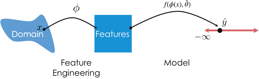
Feature engineering ⚙️

The goal of feature engineering

• Feature engineering is the act of finding transformations that transform data into effective quantitative variables.

• A feature function $\phi$ (phi, pronounced "fea") is a mapping from raw data to $d$-dimensional space, i.e. $\phi: \text{raw data} \rightarrow \mathbb{R}^d$.
  • If two observations $x_i$ and $x_j$ are "similar" in the raw data space, then $\phi(x_i)$ and $\phi(x_j)$ should also be "similar."

• A "good" choice of features depends on many factors:
  • The kind of data, i.e. quantitative, ordinal, or nominal.
  • The relationship(s) being modeled.
  • The model type, e.g. linear models, decision tree models, neural networks.

• To introduce different feature functions, we'll look at several different example datasets.

One hot encoding

• One hot encoding is a transformation that turns a categorical feature into several binary features.

• Suppose a column has $N$ unique values, $A_1$, $A_2$, ..., $A_N$. For each unique value $A_i$, we define the following feature function:

$$\phi_i(x) = \left\{\begin{array}{ll}1 & {\rm if\ } x = A_i \\ 0 & {\rm if\ } x\neq A_i \\ \end{array}\right. $$

• Note that 1 means "yes" and 0 means "no".

• One hot encoding is also called "dummy encoding", and $\phi(x)$ may also be referred to as an "indicator variable".

Example: One hot encoding 'smoker'

For each unique value of 'smoker' in our dataset, we must create a column for just that 'smoker'. (Remember, 'smoker' is 'Yes' when the table was in the smoking section of the restaurant and 'No' otherwise.)

tips.head()

	total_bill	tip	sex	smoker	day	time	size
0	3.07	1.00	Female	Yes	Sat	Dinner	1
1	18.78	3.00	Female	No	Thur	Dinner	2
2	26.59	3.41	Male	Yes	Sat	Dinner	3
3	14.26	2.50	Male	No	Thur	Lunch	2
4	21.16	3.00	Male	No	Thur	Lunch	2

tips['smoker'].value_counts()

smoker
No     151
Yes     93
Name: count, dtype: int64

(tips['smoker'] == 'Yes').astype(int).head()

0    1
1    0
2    1
3    0
4    0
Name: smoker, dtype: int64

for val in tips['smoker'].unique():
    tips[f'smoker == {val}'] = (tips['smoker'] == val).astype(int)

tips.head()

	total_bill	tip	sex	smoker	...	time	size	smoker == Yes	smoker == No
0	3.07	1.00	Female	Yes	...	Dinner	1	1	0
1	18.78	3.00	Female	No	...	Dinner	2	0	1
2	26.59	3.41	Male	Yes	...	Dinner	3	1	0
3	14.26	2.50	Male	No	...	Lunch	2	0	1
4	21.16	3.00	Male	No	...	Lunch	2	0	1

5 rows × 9 columns

Model #4: Multiple linear regression using total bill, table size, and smoker status

Now that we've converted 'smoker' to a numerical variable, we can use it as input in a regression model. Here's the model we'll try to fit:

$$\text{predicted tip} = w_0 + w_1 \cdot \text{total bill} + w_2 \cdot \text{table size} + w_3 \cdot \text{smoker == Yes}$$

Subtlety: There's no need to use both 'smoker == No' and 'smoker == Yes'. If we know the value of one, we already know the value of the other. We can use either one.

model_three = LinearRegression()
model_three.fit(tips[['total_bill', 'size', 'smoker == Yes']], tips['tip'])

LinearRegression()

In a Jupyter environment, please rerun this cell to show the HTML representation or trust the notebook.
On GitHub, the HTML representation is unable to render, please try loading this page with nbviewer.org.

The following cell gives us our $w^*$s:

model_three.intercept_, model_three.coef_

(np.float64(0.7090155167346057), array([ 0.09,  0.18, -0.08]))

Thus, our trained linear model to predict tips given total bills, table sizes, and smoker status (yes or no) is:

$$\text{predicted tip} = 0.709 + 0.094 \cdot \text{total bill} + 0.180 \cdot \text{table size} - 0.083 \cdot \text{smoker == Yes}$$

Visualizing Model #4

Our new fit model is:

$$\text{predicted tip} = 0.709 + 0.094 \cdot \text{total bill} + 0.180 \cdot \text{table size} - 0.083 \cdot \text{smoker == Yes}$$

To visualize our data and linear model, we'd need 4 dimensions:

• One for total bill
• One for table size
• One for 'smoker == Yes'.
• One for tip.

Humans can't visualize in 4D, but there may be a solution. We know that 'smoker == Yes' only has two possible values, 1 or 0, so let's look at those cases separately.

Case 1: 'smoker == Yes' is 1, meaning that the table was in the smoking section.

$$\begin{align*} \text{predicted tip} &= 0.709 + 0.094 \cdot \text{total bill} + 0.180 \cdot \text{table size} - 0.083 \cdot 1 \\ &= 0.626 + 0.094 \cdot \text{total bill} + 0.180 \cdot \text{table size} \end{align*}$$

Case 2: 'smoker == Yes' is 0, meaning that the table was not in the smoking section.

$$\begin{align*} \text{predicted tip} &= 0.709 + 0.094 \cdot \text{total bill} + 0.180 \cdot \text{table size} - 0.083 \cdot 0 \\ &= 0.709 + 0.094 \cdot \text{total bill} + 0.180 \cdot \text{table size} \end{align*}$$

Key idea: These are two parallel planes in 3D, with different $z$-intercepts!

Note that the two planes are very close to one another – you'll have to zoom in to see the difference.

# pio.renderers.default = 'plotly_mimetype+notebook' # If it doesn't render, try uncommenting this.

XX, YY = np.mgrid[0:50:2, 0:8:1]
Z_0 = model_three.intercept_ + model_three.coef_[0] * XX + model_three.coef_[1] * YY + model_three.coef_[2] * 0
Z_1 = model_three.intercept_ + model_three.coef_[0] * XX + model_three.coef_[1] * YY + model_three.coef_[2] * 1
plane_0 = go.Surface(x=XX, y=YY, z=Z_0, colorscale='Greens')
plane_1 = go.Surface(x=XX, y=YY, z=Z_1, colorscale='Purples')

fig = go.Figure(data=[plane_0, plane_1])

tips_0 = tips[tips['smoker'] == 'No']
tips_1 = tips[tips['smoker'] == 'Yes']

fig.add_trace(go.Scatter3d(x=tips_0['total_bill'], 
                           y=tips_0['size'], 
                           z=tips_0['tip'], mode='markers', marker = {'color': 'green'}))

fig.add_trace(go.Scatter3d(x=tips_1['total_bill'], 
                           y=tips_1['size'], 
                           z=tips_1['tip'], mode='markers', marker = {'color': 'purple'}))

fig.update_layout(scene = dict(
    xaxis_title='Total Bill',
    yaxis_title='Table Size',
    zaxis_title='Tip'),
  title='Tip vs. Total Bill and Table Size (Green = Non-Smoking Section, Purple = Smoking Section)',
    width=1000, height=800,
    showlegend=False)

If we want to visualize in 2D, we need to pick a single feature to place on the $x$-axis.

fig = go.Figure()
fig.add_trace(go.Scatter(x=tips['total_bill'], y=tips['tip'], 
                         mode='markers', name='Original Data'))
fig.add_trace(go.Scatter(x=tips['total_bill'], y=model_three.predict(tips[['total_bill', 'size', 'smoker == Yes']]), 
                         mode='markers', name='Predicted Tips using Total Bill, <br>Table Size, and Smoker Status'))

fig.update_layout(showlegend=True, title='Tip vs. Total Bill',
                  xaxis_title='Total Bill', yaxis_title='Tip')

Despite being a linear model, why doesn't this model look like a straight line?

Comparing Model #4 to earlier models

rmse_dict['three features'] = rmse(tips['tip'], 
                                   model_three.predict(tips[['total_bill', 'size', 'smoker == Yes']]))
rmse_dict

{'constant tip amount': np.float64(1.3807999538298952),
 'one feature: total bill': np.float64(1.0178504025697377),
 'two features': np.float64(1.007256127114662),
 'three features': np.float64(1.0064899786822128)}

Adding 'smoker == Yes' decreased the training RMSE of our model, but barely.

Reflection

tips.head()

	total_bill	tip	sex	smoker	...	time	size	smoker == Yes	smoker == No
0	3.07	1.00	Female	Yes	...	Dinner	1	1	0
1	18.78	3.00	Female	No	...	Dinner	2	0	1
2	26.59	3.41	Male	Yes	...	Dinner	3	1	0
3	14.26	2.50	Male	No	...	Lunch	2	0	1
4	21.16	3.00	Male	No	...	Lunch	2	0	1

5 rows × 9 columns

• We've one hot encoded 'smoker', but it required a for-loop.

• Is there an easy way to one hot encode all four categorical columns – 'sex', 'smoker', 'day', and 'time' – all at once, without using a for-loop?

• Yes, using sklearn.preprocessing's OneHotEncoder. More on this soon!

Question 🤔 (Answer at dsc80.com/q)

Code: grocery

(Fa23 Final Q9.1)

Every week, Lauren goes to her local grocery store and buys a varying amount of vegetable but always buys exactly one pound of meat (either beef, fish, or chicken). We use a linear regression model to predict her total grocery bill. We’ve collected a dataset containing the pounds of vegetables bought, the type of meat bought, and the total bill. Below we display the first few rows of the dataset and two plots generated using the entire training set.

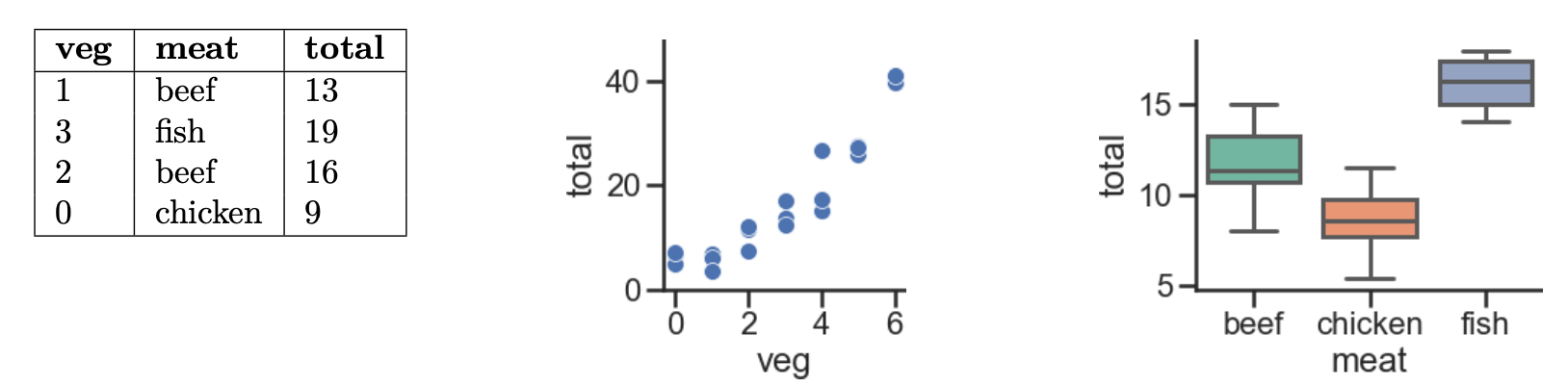
Suppose we fit the following linear regression models to predict total. Based on the data and visualizations shown above, determine whether the fitted model weights are positive (+), negative (-), or exactly 0. The notation meat=beef refers to the one-hot encoded meat column with value 1 if the original value in the meat column was beef and 0 otherwise. Likewise, meat=chicken and meat=fish are the one-hot encoded meat columns for chicken and fish, respectively.

1. $H(x) = w_0 $
2. $H(x) = w_0 + w_1 \cdot \text{veg} $
3. $H(x) = w_0 + w_1 \cdot (\text{meat=chicken}) $
4. $H(x) = w_0 + w_1 \cdot (\text{meat=beef}) + w_2 \cdot (\text{meat=chicken}) $
5. $H(x) = w_0 + w_1 \cdot (\text{meat=beef}) + w_2 \cdot (\text{meat=chicken}) + w_3 \cdot (\text{meat=fish}) $

You can copy-paste this template and then fill in your answer for each weight.

1. 
w0: ???

2.
w0: ???
w1: ???

3.
w0: ???
w1: ???

4.
w0: ???
w1: ???
w2: ???

5.
w0: ???
w1: ???
w2: ???
w3: ???

Example: Predicting ratings ⭐️

Example: Predicting ratings ⭐️

UID	AGE	STATE	HAS_BOUGHT	REVIEW	|	RATING
74	32	NY	True	"Meh."	|	✩✩
42	50	WA	True	"Worked out of the box..."	|	✩✩✩✩
57	16	CA	NULL	"Sick af..."	|	✩
...	...	...	...	...	|	...
(int)	(int)	(str)	(bool)	(str)	|	(str)

• We want to build a classifier that predicts 'RATING' using the above features.

• Why can't we build a model right away? What must we do so that we can build a model?

• Some issues: missing values, emojis and strings instead of numbers, irrelevant columns.

Uninformative features

• 'UID' was likely used to join the user information (e.g., 'AGE' and 'STATE') with some reviews dataset.

• Even though 'UID's are stored as numbers, the numerical value of a user's 'UID' won't help us predict their 'RATING'.

• If we include the 'UID' feature, our model will find whatever patterns it can between 'UID's and 'RATING's in the training (observed data).
  • This will lead to a lower training RMSE.

• However, since there is truly no relationship between 'UID' and 'RATING', this will lead to worse model performance on unseen data (bad).

Dropping features

There are certain scenarios where manually dropping features might be helpful:

1. When the features do not contain information associated with the prediction task.
2. When the feature is not available at prediction time.

• The goal of building a model to predict 'RATING's is so that we can predict 'RATING's for users who haven't actually made a 'RATING' yet.

• As such, our model should only depend on features that we would know before the user makes their 'RATING'.

• For instance, if a user only enters a 'REVIEW' after entering a 'RATING', we shouldn't use their 'REVIEW' to predict their 'RATING'.

Encoding ordinal features

UID	AGE	STATE	HAS_BOUGHT	REVIEW	|	RATING
74	32	NY	True	"Meh."	|	✩✩
42	50	WA	True	"Worked out of the box..."	|	✩✩✩✩
57	16	CA	NULL	"Sick af..."	|	✩
...	...	...	...	...	|	...
(int)	(int)	(str)	(bool)	(str)	|	(str)

How do we encode the 'RATING' column, an ordinal variable, as a quantitative variable?

• Transformation: Replace "number of ✩" with "number".
  • This is an ordinal encoding, a transformation that maps ordinal values to the positive integers in a way that preserves order.
  • Example: (freshman, sophomore, junior, senior) -> (0, 1, 2, 3).
  • Important: This transformation preserves "distances" between ratings.

ordinal_enc = {
    '✩': 1,
    '✩✩': 2,
    '✩✩✩': 3,
    '✩✩✩✩': 4,
    '✩✩✩✩✩': 5,
}
ordinal_enc

{'✩': 1, '✩✩': 2, '✩✩✩': 3, '✩✩✩✩': 4, '✩✩✩✩✩': 5}

ratings = pd.DataFrame().assign(rating=['✩', '✩✩', '✩✩✩', '✩✩', '✩✩✩', '✩', '✩✩✩', '✩✩✩✩', '✩✩✩✩✩'])
ratings

	rating
0	✩
1	✩✩
2	✩✩✩
...	...
6	✩✩✩
7	✩✩✩✩
8	✩✩✩✩✩

9 rows × 1 columns

ratings['rating'].map(ordinal_enc)

0    1
1    2
2    3
    ..
6    3
7    4
8    5
Name: rating, Length: 9, dtype: int64

Encoding nominal features

UID	AGE	STATE	HAS_BOUGHT	REVIEW	|	RATING
74	32	NY	True	"Meh."	|	✩✩
42	50	WA	True	"Worked out of the box..."	|	✩✩✩✩
57	16	CA	NULL	"Sick af..."	|	✩
...	...	...	...	...	|	...
(int)	(int)	(str)	(bool)	(str)	|	(str)

How do we encode the 'STATE' column, a nominal variable, as a quantitative variable? In other words, how do we turn 'STATE's into meaningful numbers?

• Question: Why can't we use an ordinal encoding, e.g. NY -> 0, WA -> 1?

• Answer: There is no inherent ordering to states, e.g. WA is not inherently "more" of anything than NY.

• We've already seen the correct strategy: one hot encoding.

Example: Horsepower 🚗

The following dataset, built into the seaborn plotting library, contains various information about (older) cars.

mpg = sns.load_dataset('mpg').dropna()
mpg.head()

	mpg	cylinders	displacement	horsepower	...	acceleration	model_year	origin	name
0	18.0	8	307.0	130.0	...	12.0	70	usa	chevrolet chevelle malibu
1	15.0	8	350.0	165.0	...	11.5	70	usa	buick skylark 320
2	18.0	8	318.0	150.0	...	11.0	70	usa	plymouth satellite
3	16.0	8	304.0	150.0	...	12.0	70	usa	amc rebel sst
4	17.0	8	302.0	140.0	...	10.5	70	usa	ford torino

5 rows × 9 columns

We really do mean old:

mpg['model_year'].value_counts()

model_year
73    40
78    36
76    34
      ..
71    27
80    27
74    26
Name: count, Length: 13, dtype: int64

Let's investigate the relationship between 'horsepower' and 'mpg'.

The relationship between 'horsepower' and 'mpg'

px.scatter(mpg, x='horsepower', y='mpg')

• It appears that there is a negative association between 'horsepower' and 'mpg', though it's not quite linear.

• Let's try and fit a simple linear model that uses 'horsepower' to predict 'mpg' and see what happens.

Predicting 'mpg' using 'horsepower'

car_model = LinearRegression()
car_model.fit(mpg[['horsepower']], mpg['mpg'])

LinearRegression()

In a Jupyter environment, please rerun this cell to show the HTML representation or trust the notebook.
On GitHub, the HTML representation is unable to render, please try loading this page with nbviewer.org.

What do our predictions look like?

hp_points = pd.DataFrame({'horsepower': [25, 225]})
fig = px.scatter(mpg, x='horsepower', y='mpg')
fig.add_trace(go.Scatter(
    x=hp_points['horsepower'],
    y=car_model.predict(hp_points),
    mode='lines',
    name='Predicted MPG using Horsepower'
))

Our regression line doesn't capture the curvature in the relationship between 'horsepower' and 'mpg'.

Let's look at the residuals:

res = mpg.assign(
    Predictions=car_model.predict(mpg[['horsepower']]),
    Residuals=mpg['mpg'] - car_model.predict(mpg[['horsepower']]),
)
fig = px.scatter(res, x='Predictions', y='Residuals')
fig.add_hline(0, line_width=3, opacity=1)

car_model.score(mpg[['horsepower']], mpg['mpg'])

0.6059482578894351

Linearization

The Tukey Mosteller Bulge Diagram helps us pick which transformations to apply to data in order to linearize it.

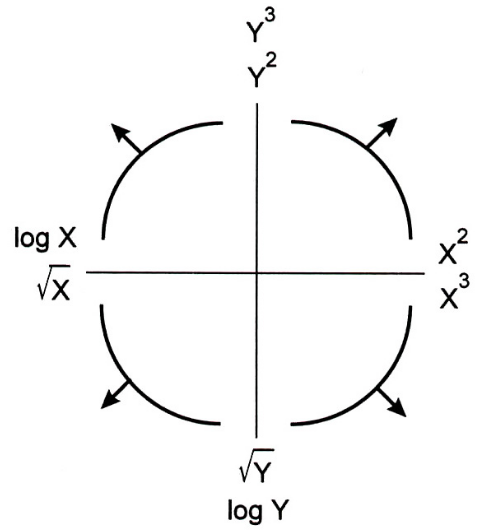
The bottom-left quadrant appears to match the shape of the scatter plot between 'horsepower' and 'mpg' the best – let's try taking the log of 'horsepower' ($X$).

mpg['log hp'] = np.log(mpg['horsepower'])

What does our data look like now?

px.scatter(mpg, x='log hp', y='mpg')

Predicting 'mpg' using log('horsepower')

Let's fit another linear model.

car_model_log = LinearRegression()
car_model_log.fit(mpg[['log hp']], mpg['mpg'])

LinearRegression()

In a Jupyter environment, please rerun this cell to show the HTML representation or trust the notebook.
On GitHub, the HTML representation is unable to render, please try loading this page with nbviewer.org.

What do our predictions look like now?

fig = px.scatter(mpg, x='log hp', y='mpg')
log_hp_points = pd.DataFrame({'log hp': [3.7, 5.5]})
fig = px.scatter(mpg, x='log hp', y='mpg')
fig.add_trace(go.Scatter(
    x=log_hp_points['log hp'],
    y=car_model_log.predict(log_hp_points),
    mode='lines',
    name='Predicted MPG using log(Horsepower)'
))

The fit looks a bit better! How about the $R^2$?

car_model_log.score(mpg[['log hp']], mpg['mpg'])

0.6683347641192137

Also a bit better!

What do our predictions look like on the original, non-transformed scatter plot? Let's see:

fig = px.scatter(mpg, x='horsepower', y='mpg')
fig.add_trace(
    go.Scatter(
        x=mpg['horsepower'], 
        y=car_model_log.intercept_ + car_model_log.coef_[0] * np.log(mpg['horsepower']),  
        mode='markers', name='Predicted MPG using log(Horsepower)'
    )
)
fig

Our predictions that used $\log(\text{Horsepower})$ as an input don't fall on a straight line. We shouldn't expect them to; the red dots come from:

$$\text{Predicted MPG} = 108.698 - 18.582 \cdot \log(\text{Horsepower})$$

car_model_log.intercept_, car_model_log.coef_

(np.float64(108.69970699574483), array([-18.58]))

Quantitative scaling

Until now, feature transformations we've discussed so far have involved converting categorical variables into quantitative variables. However, our log transformation was an example of transforming a quantitative variable into a new quantitative variable; this practice is called quantitative scaling.

• Standardization: $x_i \rightarrow \frac{x_i - \bar{x}}{\sigma_x}$.
• Linearization via a non-linear transformation: e.g. $\text{log}$ and $\text{sqrt}$. See Lab 8 for more.
• Discretization: Convert data into percentiles (or more generally, quantiles).

Question 🤔 (Answer at dsc80.com/q)

Code: q14

Ask a question about something you feel unsure about so far.

The modeling process

The modeling process

1. Create, or engineer, features to best reflect the "meaning" behind data.

2. Choose a model that is appropriate to capture the relationships between features ($X$) and the target/response ($y$).

3. Choose a loss function, e.g. squared loss.

4. Fit the model: that is, minimize empirical risk to find optimal model parameters $w^*$.

5. Evaluate the model, e.g. using RMSE or $R^2$.

We can perform all of the above directly in sklearn!

preprocessing and linear_models

For the feature engineering step of the modeling pipeline, we will use sklearn's preprocessing module.

For the model creation step of the modeling pipeline, we will use sklearn's linear_model module, as we've already seen. linear_model.LinearRegression is an example of an estimator class.

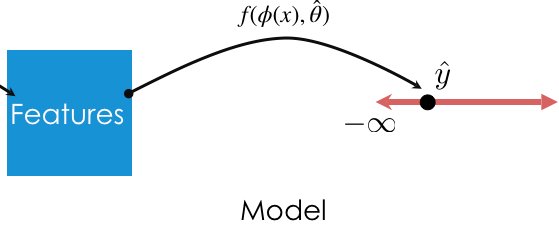
Transformers in sklearn

Transformer classes

• Transformers take in "raw" data and output "processed" data. They are used for creating features.

• The input to a transformer should be a multi-dimensional numpy array.
  • Inputs can be DataFrames, but sklearn only looks at the values (i.e. it calls to_numpy() on input DataFrames).

• The output of a transformer is a numpy array (never a DataFrame or Series).

• Transformers, like most relevant features of sklearn, are classes, not functions, meaning you need to instantiate them and call their methods.

Example: Predicting tips 🧑‍🍳

We'll continue working with our trusty tips dataset.

tips.head()

	total_bill	tip	sex	smoker	...	time	size	smoker == Yes	smoker == No
0	3.07	1.00	Female	Yes	...	Dinner	1	1	0
1	18.78	3.00	Female	No	...	Dinner	2	0	1
2	26.59	3.41	Male	Yes	...	Dinner	3	1	0
3	14.26	2.50	Male	No	...	Lunch	2	0	1
4	21.16	3.00	Male	No	...	Lunch	2	0	1

5 rows × 9 columns

Example transformer: Binarizer

The Binarizer transformer allows us to map a quantitative sequence to a sequence of 1s and 0s, depending on whether values are above or below a threshold.

Property	Example	Description
Initialize with parameters	binar = Binarizer(thresh)	set x=1 if x > thresh, else 0
Transform data in a dataset	feat = binar.transform(data)	Binarize all columns in data

First, we need to import the relevant class from sklearn.preprocessing. (Tip: import just the relevant classes you need from sklearn.)

from sklearn.preprocessing import Binarizer

Let's try binarizing 'total_bill'. We'll say a "large" bill is one that is strictly greater than $20.

tips['total_bill'].head()

0     3.07
1    18.78
2    26.59
3    14.26
4    21.16
Name: total_bill, dtype: float64

First, we initialize a Binarizer object with the threshold we want.

bi = Binarizer(threshold=20)

Then, we call bi's transform method and pass it the data we'd like to transform. Note that its input and output are both 2D.

transformed_bills = bi.transform(tips[['total_bill']]) # Must give transform a 2D array/DataFrame.
transformed_bills[:5]

/Users/watson-parris/miniconda3/envs/dsc80/lib/python3.12/site-packages/sklearn/base.py:486: UserWarning:

X has feature names, but Binarizer was fitted without feature names

array([[0.],
       [0.],
       [1.],
       [0.],
       [1.]])

Example transformer: StandardScaler

• StandardScaler standardizes data using the mean and standard deviation of the data.

$$z(x_i) = \frac{x_i - \text{mean of } x}{\text{SD of } x}$$

• Unlike Binarizer, StandardScaler requires some knowledge (mean and SD) of the dataset before transforming.

• As such, we need to fit an StandardScaler transformer before we can use the transform method.

• Typical usage: fit transformer on a sample, use that fit transformer to transform future data.

Example transformer: StandardScaler

It only makes sense to standardize the already-quantitative features of tips, so let's select just those.

tips_quant = tips[['total_bill', 'size']]
tips_quant.head()

	total_bill	size
0	3.07	1
1	18.78	2
2	26.59	3
3	14.26	2
4	21.16	2

Let's initialize a StandardScaler object.

from sklearn.preprocessing import StandardScaler

stdscaler = StandardScaler()

Note that the following does not work! The error message is very helpful.

stdscaler.transform(tips_quant)

---------------------------------------------------------------------------
NotFittedError                            Traceback (most recent call last)
Cell In[50], line 1
----> 1 stdscaler.transform(tips_quant)

File ~/miniconda3/envs/dsc80/lib/python3.12/site-packages/sklearn/utils/_set_output.py:316, in _wrap_method_output.<locals>.wrapped(self, X, *args, **kwargs)
    314 @wraps(f)
    315 def wrapped(self, X, *args, **kwargs):
--> 316     data_to_wrap = f(self, X, *args, **kwargs)
    317     if isinstance(data_to_wrap, tuple):
    318         # only wrap the first output for cross decomposition
    319         return_tuple = (
    320             _wrap_data_with_container(method, data_to_wrap[0], X, self),
    321             *data_to_wrap[1:],
    322         )

File ~/miniconda3/envs/dsc80/lib/python3.12/site-packages/sklearn/preprocessing/_data.py:1042, in StandardScaler.transform(self, X, copy)
   1027 def transform(self, X, copy=None):
   1028     """Perform standardization by centering and scaling.
   1029 
   1030     Parameters
   (...)
   1040         Transformed array.
   1041     """
-> 1042     check_is_fitted(self)
   1044     copy = copy if copy is not None else self.copy
   1045     X = self._validate_data(
   1046         X,
   1047         reset=False,
   (...)
   1052         force_all_finite="allow-nan",
   1053     )

File ~/miniconda3/envs/dsc80/lib/python3.12/site-packages/sklearn/utils/validation.py:1661, in check_is_fitted(estimator, attributes, msg, all_or_any)
   1658     raise TypeError("%s is not an estimator instance." % (estimator))
   1660 if not _is_fitted(estimator, attributes, all_or_any):
-> 1661     raise NotFittedError(msg % {"name": type(estimator).__name__})

NotFittedError: This StandardScaler instance is not fitted yet. Call 'fit' with appropriate arguments before using this estimator.

Instead, we need to first call the fit method on stdscaler.

# This is like saying "determine the mean and SD of each column in tips_quant".
stdscaler.fit(tips_quant)

StandardScaler()

In a Jupyter environment, please rerun this cell to show the HTML representation or trust the notebook.
On GitHub, the HTML representation is unable to render, please try loading this page with nbviewer.org.

Now, transform will work.

# First column is 'total_bill', second column is 'size'.
tips_quant_z = stdscaler.transform(tips_quant)
tips_quant_z[:5]

array([[-1.88, -1.65],
       [-0.11, -0.6 ],
       [ 0.77,  0.45],
       [-0.62, -0.6 ],
       [ 0.15, -0.6 ]])

We can also access the mean and variance stdscaler computed for each column:

stdscaler.mean_

array([19.79,  2.57])

stdscaler.var_

array([78.93,  0.9 ])

Note that we can call transform on DataFrames other than tips_quant. We will do this often – fit a transformer on one dataset (training data) and use it to transform other datasets (test data).

stdscaler.transform(tips_quant.sample(5))

array([[ 0.97, -0.6 ],
       [-0.28, -0.6 ],
       [ 1.19,  1.51],
       [-0.49, -0.6 ],
       [ 0.65,  1.51]])

💡 Pro-Tip: Using .fit_transform

The .fit_transform method will fit the transformer and then transform the data in one go.

stdscaler.fit_transform(tips_quant)

array([[-1.88, -1.65],
       [-0.11, -0.6 ],
       [ 0.77,  0.45],
       ...,
       [-0.26, -0.6 ],
       [-1.09, -0.6 ],
       [-0.32,  0.45]])

StandardScaler summary

Property	Example	Description
Initialize with parameters	stdscaler = StandardScaler()	z-score the data (no parameters)
Fit the transformer	stdscaler.fit(X)	Compute the mean and SD of X
Transform data in a dataset	feat = stdscaler.transform(X_new)	z-score X_new with mean and SD of X
Fit and transform	stdscaler.fit_transform(X)	Compute the mean and SD of X, then z-score X

Example transformer: OneHotEncoder

Let's keep just the categorical columns in tips.

tips_cat = tips[['sex', 'smoker', 'day', 'time']]
tips_cat.head()

	sex	smoker	day	time
0	Female	Yes	Sat	Dinner
1	Female	No	Thur	Dinner
2	Male	Yes	Sat	Dinner
3	Male	No	Thur	Lunch
4	Male	No	Thur	Lunch

Like StdScaler, we will need to fit our OneHotEncoder transformer before it can transform anything.

from sklearn.preprocessing import OneHotEncoder

ohe = OneHotEncoder()
ohe.fit(tips_cat)

OneHotEncoder()

In a Jupyter environment, please rerun this cell to show the HTML representation or trust the notebook.
On GitHub, the HTML representation is unable to render, please try loading this page with nbviewer.org.

When we try and transform, we get a result we might not expect.

ohe.transform(tips_cat)

<Compressed Sparse Row sparse matrix of dtype 'float64'
	with 976 stored elements and shape (244, 10)>

Since the resulting matrix is sparse – most of its elements are 0 – sklearn uses a more efficient representation than a regular numpy array. We can convert to a regular (dense) array:

ohe.transform(tips_cat).toarray()

array([[1., 0., 0., ..., 0., 1., 0.],
       [1., 0., 1., ..., 1., 1., 0.],
       [0., 1., 0., ..., 0., 1., 0.],
       ...,
       [1., 0., 1., ..., 1., 0., 1.],
       [0., 1., 1., ..., 0., 1., 0.],
       [1., 0., 1., ..., 0., 1., 0.]])

Notice that the column names from tips_cat are no longer stored anywhere (remember, fit converts the input to a numpy array before proceeding).

We can use the get_feature_names_out method on ohe to access the names of the one-hot-encoded columns, though:

ohe.get_feature_names_out() # x0, x1, x2, and x3 correspond to column names in tips_cat.

array(['sex_Female', 'sex_Male', 'smoker_No', 'smoker_Yes', 'day_Fri',
       'day_Sat', 'day_Sun', 'day_Thur', 'time_Dinner', 'time_Lunch'],
      dtype=object)

pd.DataFrame(ohe.transform(tips_cat).toarray(), 
             columns=ohe.get_feature_names_out()) # If we need a DataFrame back, for some reason.

	sex_Female	sex_Male	smoker_No	smoker_Yes	...	day_Sun	day_Thur	time_Dinner	time_Lunch
0	1.0	0.0	0.0	1.0	...	0.0	0.0	1.0	0.0
1	1.0	0.0	1.0	0.0	...	0.0	1.0	1.0	0.0
2	0.0	1.0	0.0	1.0	...	0.0	0.0	1.0	0.0
...	...	...	...	...	...	...	...	...	...
241	1.0	0.0	1.0	0.0	...	0.0	1.0	0.0	1.0
242	0.0	1.0	1.0	0.0	...	0.0	0.0	1.0	0.0
243	1.0	0.0	1.0	0.0	...	0.0	0.0	1.0	0.0

244 rows × 10 columns

Question 🤔 (Answer at dsc80.com/q)

Code: ohe

Suppose we have a training set X_train with labels y_train, and we have a test set X_test with labels y_test. If we want to use OHE on the day column, we will use ohe.fit_transform(X_train), but we will NOT do ohe.fit_transform(X_test). Instead, we will ONLY do ohe.transform(X_test). Why?

Summary, next time

Summary

• To transform a categorical nominal variable into a quantitative variable, use one hot encoding.
• To transform a categorical ordinal variable into a quantitative variable, use an ordinal encoding.
• Quantitative feature transformations allow us to use linear models to model non-linear data.

Next time

• Pipelines that allow us to easily combine these steps
• Multicollinearity.
• Generalization.