from dsc80_utils import *
import lec15_util as util
Agenda 📆
- Pipelines.
- Multicollinearity.
- Generalization.
- Bias and variance.
- Train-test splits.
Pipelines
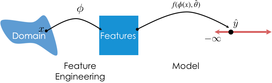
So far, we've used transformers for feature engineering and models for prediction. We can combine these steps into a single Pipeline.
Pipelines in sklearn
- Pipeline allows you to sequentially apply a list of transformers to preprocess the data and, if desired, conclude the sequence with a final predictor for predictive modeling.
- General template:
pl = Pipeline([trans_1, trans_2, ..., model])- Note that the
modelis optional.
- Note that the
- Once a
Pipelineis instantiated, you can fit all steps (transformers and model) usingpl.fit(X, y).
- To make predictions using raw, untransformed data, use
pl.predict(X).
- The actual list we provide
Pipelinewith must be a list of tuples, where- The first element is a "name" (that we choose) for the step.
- The second element is a transformer or estimator instance.
Our first Pipeline
Let's build a Pipeline that:
- One hot encodes the categorical features in
tips. - Fits a regression model on the one hot encoded data.
tips = px.data.tips()
tips_cat = tips[['sex', 'smoker', 'day', 'time']]
tips_cat.head()
| sex | smoker | day | time | |
|---|---|---|---|---|
| 0 | Female | No | Sun | Dinner |
| 1 | Male | No | Sun | Dinner |
| 2 | Male | No | Sun | Dinner |
| 3 | Male | No | Sun | Dinner |
| 4 | Female | No | Sun | Dinner |
from sklearn.pipeline import Pipeline
from sklearn.preprocessing import OneHotEncoder
from sklearn.linear_model import LinearRegression
pl = Pipeline([
('one-hot', OneHotEncoder()),
('lin-reg', LinearRegression())
])
Now that pl is instantiated, we fit it the same way we would fit the individual steps.
pl.fit(tips_cat, tips['tip'])
Pipeline(steps=[('one-hot', OneHotEncoder()), ('lin-reg', LinearRegression())])In a Jupyter environment, please rerun this cell to show the HTML representation or trust the notebook. On GitHub, the HTML representation is unable to render, please try loading this page with nbviewer.org.
Pipeline(steps=[('one-hot', OneHotEncoder()), ('lin-reg', LinearRegression())])OneHotEncoder()
LinearRegression()
Now, to make predictions using raw data, all we need to do is use pl.predict:
pl.predict(tips_cat.iloc[:5])
array([3.1 , 3.27, 3.27, 3.27, 3.1 ])
pl performs both feature transformation and prediction with just a single call to predict!
We can access individual "steps" of a Pipeline through the named_steps attribute:
pl.named_steps
{'one-hot': OneHotEncoder(), 'lin-reg': LinearRegression()}
pl.named_steps['one-hot'].transform(tips_cat).toarray()
array([[1., 0., 1., ..., 0., 1., 0.],
[0., 1., 1., ..., 0., 1., 0.],
[0., 1., 1., ..., 0., 1., 0.],
...,
[0., 1., 0., ..., 0., 1., 0.],
[0., 1., 1., ..., 0., 1., 0.],
[1., 0., 1., ..., 1., 1., 0.]])
pl.named_steps['one-hot'].get_feature_names_out()
array(['sex_Female', 'sex_Male', 'smoker_No', 'smoker_Yes', 'day_Fri',
'day_Sat', 'day_Sun', 'day_Thur', 'time_Dinner', 'time_Lunch'],
dtype=object)
pl.named_steps['lin-reg'].coef_
array([-0.09, 0.09, -0.04, 0.04, -0.2 , -0.13, 0.14, 0.19, 0.25,
-0.25])
pl also has a score method, the same way a fit LinearRegression instance does:
# Why is this so low?
pl.score(tips_cat, tips['tip'])
0.02749679020147555
More sophisticated Pipelines
- In the previous example, we one hot encoded every input column. What if we want to perform different transformations on different columns?
- Solution: Use a
ColumnTransformer.- Instantiate a
ColumnTransformerusing a list of tuples, where:- The first element is a "name" we choose for the transformer.
- The second element is a transformer instance (e.g.
OneHotEncoder()). - The third element is a list of relevant column names.
- Instantiate a
Planning our first ColumnTransformer
from sklearn.compose import ColumnTransformer
Let's perform different transformations on the quantitative and categorical features of tips (note that we are not transforming 'tip').
tips_features = tips.drop('tip', axis=1)
tips_features.head()
| total_bill | sex | smoker | day | time | size | |
|---|---|---|---|---|---|---|
| 0 | 16.99 | Female | No | Sun | Dinner | 2 |
| 1 | 10.34 | Male | No | Sun | Dinner | 3 |
| 2 | 21.01 | Male | No | Sun | Dinner | 3 |
| 3 | 23.68 | Male | No | Sun | Dinner | 2 |
| 4 | 24.59 | Female | No | Sun | Dinner | 4 |
- We will leave the
'total_bill'column untouched.
- To the
'size'column, we will apply theBinarizertransformer with a threshold of 2 (big tables vs. small tables).
- To the categorical columns, we will apply the
OneHotEncodertransformer.
- In essence, we will create a transformer that reproduces the following DataFrame:
| size | x0_Female | x0_Male | x1_No | x1_Yes | x2_Fri | x2_Sat | x2_Sun | x2_Thur | x3_Dinner | x3_Lunch | total_bill | |
|---|---|---|---|---|---|---|---|---|---|---|---|---|
| 0 | 0 | 1.0 | 0.0 | 1.0 | 0.0 | 0.0 | 0.0 | 1.0 | 0.0 | 1.0 | 0.0 | 16.99 |
| 1 | 1 | 0.0 | 1.0 | 1.0 | 0.0 | 0.0 | 0.0 | 1.0 | 0.0 | 1.0 | 0.0 | 10.34 |
| 2 | 1 | 0.0 | 1.0 | 1.0 | 0.0 | 0.0 | 0.0 | 1.0 | 0.0 | 1.0 | 0.0 | 21.01 |
| 3 | 0 | 0.0 | 1.0 | 1.0 | 0.0 | 0.0 | 0.0 | 1.0 | 0.0 | 1.0 | 0.0 | 23.68 |
| 4 | 1 | 1.0 | 0.0 | 1.0 | 0.0 | 0.0 | 0.0 | 1.0 | 0.0 | 1.0 | 0.0 | 24.59 |
Building a Pipeline using a ColumnTransformer
Let's start by creating our ColumnTransformer.
from sklearn.preprocessing import Binarizer
preproc = ColumnTransformer(
transformers=[
('size', Binarizer(threshold=2), ['size']),
('categorical_cols', OneHotEncoder(), ['sex', 'smoker', 'day', 'time'])
],
# Specify what to do with all other columns ('total_bill' here) – drop or passthrough.
remainder='passthrough',
# Keep original dtypes for remaining columns
force_int_remainder_cols=False,
)
Now, let's create a Pipeline using preproc as a transformer, and fit it:
pl = Pipeline([
('preprocessor', preproc),
('lin-reg', LinearRegression())
])
pl.fit(tips_features, tips['tip'])
Pipeline(steps=[('preprocessor',
ColumnTransformer(force_int_remainder_cols=False,
remainder='passthrough',
transformers=[('size',
Binarizer(threshold=2),
['size']),
('categorical_cols',
OneHotEncoder(),
['sex', 'smoker', 'day',
'time'])])),
('lin-reg', LinearRegression())])In a Jupyter environment, please rerun this cell to show the HTML representation or trust the notebook. On GitHub, the HTML representation is unable to render, please try loading this page with nbviewer.org.
Pipeline(steps=[('preprocessor',
ColumnTransformer(force_int_remainder_cols=False,
remainder='passthrough',
transformers=[('size',
Binarizer(threshold=2),
['size']),
('categorical_cols',
OneHotEncoder(),
['sex', 'smoker', 'day',
'time'])])),
('lin-reg', LinearRegression())])ColumnTransformer(force_int_remainder_cols=False, remainder='passthrough',
transformers=[('size', Binarizer(threshold=2), ['size']),
('categorical_cols', OneHotEncoder(),
['sex', 'smoker', 'day', 'time'])])['size']
Binarizer(threshold=2)
['sex', 'smoker', 'day', 'time']
OneHotEncoder()
['total_bill']
passthrough
LinearRegression()
Prediction is as easy as calling predict:
tips_features.head()
| total_bill | sex | smoker | day | time | size | |
|---|---|---|---|---|---|---|
| 0 | 16.99 | Female | No | Sun | Dinner | 2 |
| 1 | 10.34 | Male | No | Sun | Dinner | 3 |
| 2 | 21.01 | Male | No | Sun | Dinner | 3 |
| 3 | 23.68 | Male | No | Sun | Dinner | 2 |
| 4 | 24.59 | Female | No | Sun | Dinner | 4 |
# Note that we fit the Pipeline using tips_features, not tips_features.head()!
pl.predict(tips_features.head())
array([2.74, 2.32, 3.37, 3.37, 3.75])
Aside: FunctionTransformer
A transformer you'll often use as part of a ColumnTransformer is the FunctionTransformer, which enables you to use your own functions on entire columns. Think of it as the sklearn equivalent of apply.
from sklearn.preprocessing import FunctionTransformer
f = FunctionTransformer(np.sqrt)
f.transform([1, 2, 3])
array([1. , 1.41, 1.73])
💡 Pro-Tip: Using make_pipeline and make_column_transformer
Instead of using Pipeline and ColumnTransformer classes directly, scikit-learn provides nifty shortcut methods called make_pipeline and make_column_transformer:
# Old code
preproc = ColumnTransformer(
transformers=[
('size', Binarizer(threshold=2), ['size']),
('categorical_cols', OneHotEncoder(), ['sex', 'smoker', 'day', 'time'])
],
remainder='passthrough'
)
pl = Pipeline([
('preprocessor', preproc),
('lin-reg', LinearRegression())
])
pl
Pipeline(steps=[('preprocessor',
ColumnTransformer(remainder='passthrough',
transformers=[('size',
Binarizer(threshold=2),
['size']),
('categorical_cols',
OneHotEncoder(),
['sex', 'smoker', 'day',
'time'])])),
('lin-reg', LinearRegression())])In a Jupyter environment, please rerun this cell to show the HTML representation or trust the notebook. On GitHub, the HTML representation is unable to render, please try loading this page with nbviewer.org.
Pipeline(steps=[('preprocessor',
ColumnTransformer(remainder='passthrough',
transformers=[('size',
Binarizer(threshold=2),
['size']),
('categorical_cols',
OneHotEncoder(),
['sex', 'smoker', 'day',
'time'])])),
('lin-reg', LinearRegression())])ColumnTransformer(remainder='passthrough',
transformers=[('size', Binarizer(threshold=2), ['size']),
('categorical_cols', OneHotEncoder(),
['sex', 'smoker', 'day', 'time'])])['size']
Binarizer(threshold=2)
['sex', 'smoker', 'day', 'time']
OneHotEncoder()
passthrough
LinearRegression()
from sklearn.pipeline import make_pipeline
from sklearn.compose import make_column_transformer
preproc = make_column_transformer(
(Binarizer(threshold=2), ['size']),
(OneHotEncoder(), ['sex', 'smoker', 'day', 'time']),
remainder='passthrough',
)
pl = make_pipeline(preproc, LinearRegression())
# Notice that the steps in the pipeline and column transformer are
# automatically named
pl
Pipeline(steps=[('columntransformer',
ColumnTransformer(remainder='passthrough',
transformers=[('binarizer',
Binarizer(threshold=2),
['size']),
('onehotencoder',
OneHotEncoder(),
['sex', 'smoker', 'day',
'time'])])),
('linearregression', LinearRegression())])In a Jupyter environment, please rerun this cell to show the HTML representation or trust the notebook. On GitHub, the HTML representation is unable to render, please try loading this page with nbviewer.org.
Pipeline(steps=[('columntransformer',
ColumnTransformer(remainder='passthrough',
transformers=[('binarizer',
Binarizer(threshold=2),
['size']),
('onehotencoder',
OneHotEncoder(),
['sex', 'smoker', 'day',
'time'])])),
('linearregression', LinearRegression())])ColumnTransformer(remainder='passthrough',
transformers=[('binarizer', Binarizer(threshold=2), ['size']),
('onehotencoder', OneHotEncoder(),
['sex', 'smoker', 'day', 'time'])])['size']
Binarizer(threshold=2)
['sex', 'smoker', 'day', 'time']
OneHotEncoder()
passthrough
LinearRegression()
An example Pipeline
One of the transformers we used was the StandardScaler transformer, which standardizes columns.
$$z(x_i) = \frac{x_i - \text{mean of } x}{\text{SD of } x}$$
Let's build a Pipeline that:
- Takes in the
'total_bill'and'size'features oftips. - Standardizes those features.
- Uses the resulting standardized features to fit a linear model that predicts
'tip'.
# Let's define these once, since we'll use them repeatedly.
X = tips[['total_bill', 'size']]
y = tips['tip']
from sklearn.preprocessing import StandardScaler
model_with_std = make_pipeline(
StandardScaler(),
LinearRegression(),
)
model_with_std.fit(X, y)
Pipeline(steps=[('standardscaler', StandardScaler()),
('linearregression', LinearRegression())])In a Jupyter environment, please rerun this cell to show the HTML representation or trust the notebook. On GitHub, the HTML representation is unable to render, please try loading this page with nbviewer.org.
Pipeline(steps=[('standardscaler', StandardScaler()),
('linearregression', LinearRegression())])StandardScaler()
LinearRegression()
How well does our model do? We can compute its $R^2$ and RMSE.
model_with_std.score(X, y)
0.46786930879612587
from sklearn.metrics import root_mean_squared_error
root_mean_squared_error(y, model_with_std.predict(X))
np.float64(1.007256127114662)
Does this model perform any better than one that doesn't standardize its features? Let's find out.
model_without_std = LinearRegression()
model_without_std.fit(X, y)
LinearRegression()In a Jupyter environment, please rerun this cell to show the HTML representation or trust the notebook.
On GitHub, the HTML representation is unable to render, please try loading this page with nbviewer.org.
LinearRegression()
model_without_std.score(X, y)
0.46786930879612587
root_mean_squared_error(y, model_without_std.predict(X))
np.float64(1.007256127114662)
No!
The purpose of standardizing features
If you're performing "vanilla" linear regression – that is, using the LinearRegression object – then standardizing your features will not change your model's error.
- There are other models where standardizing your features will improve performance, because the methods assume features are standardized.
- There is a benefit to standardizing features when performing vanilla linear regression, as we saw in DSC 40A: the features are brought to the same scale, so the coefficients can be compared directly.
# Total bill, table size.
model_without_std.coef_
array([0.09, 0.19])
# Total bill, table size.
model_with_std.named_steps['linearregression'].coef_
array([0.82, 0.18])
Aside: Pipelines of just transformers
If you want to apply multiple transformations to the same column in a dataset, you can create a Pipeline just for that column.
For example, suppose we want to:
- One hot encode the
'sex','smoker', and'time'columns. - One hot encode the
'day'column, but as either'Weekday','Sat', or'Sun'. - Binarize the
'size'column.
Here's how we might do that:
def is_weekend(s):
# The input to is_weekend is a Series!
return s.replace({'Thur': 'Weekday', 'Fri': 'Weekday'})
pl_day = make_pipeline(
FunctionTransformer(is_weekend),
OneHotEncoder(),
)
col_trans = make_column_transformer(
(pl_day, ['day']),
(OneHotEncoder(drop='first'), ['sex', 'smoker', 'time']),
(Binarizer(threshold=2), ['size']),
remainder='passthrough',
force_int_remainder_cols=False,
)
pl = make_pipeline(
col_trans,
LinearRegression(),
)
pl.fit(tips.drop('tip', axis=1), tips['tip'])
Pipeline(steps=[('columntransformer',
ColumnTransformer(force_int_remainder_cols=False,
remainder='passthrough',
transformers=[('pipeline',
Pipeline(steps=[('functiontransformer',
FunctionTransformer(func=<function is_weekend at 0x283024180>)),
('onehotencoder',
OneHotEncoder())]),
['day']),
('onehotencoder',
OneHotEncoder(drop='first'),
['sex', 'smoker', 'time']),
('binarizer',
Binarizer(threshold=2),
['size'])])),
('linearregression', LinearRegression())])In a Jupyter environment, please rerun this cell to show the HTML representation or trust the notebook. On GitHub, the HTML representation is unable to render, please try loading this page with nbviewer.org.
Pipeline(steps=[('columntransformer',
ColumnTransformer(force_int_remainder_cols=False,
remainder='passthrough',
transformers=[('pipeline',
Pipeline(steps=[('functiontransformer',
FunctionTransformer(func=<function is_weekend at 0x283024180>)),
('onehotencoder',
OneHotEncoder())]),
['day']),
('onehotencoder',
OneHotEncoder(drop='first'),
['sex', 'smoker', 'time']),
('binarizer',
Binarizer(threshold=2),
['size'])])),
('linearregression', LinearRegression())])ColumnTransformer(force_int_remainder_cols=False, remainder='passthrough',
transformers=[('pipeline',
Pipeline(steps=[('functiontransformer',
FunctionTransformer(func=<function is_weekend at 0x283024180>)),
('onehotencoder',
OneHotEncoder())]),
['day']),
('onehotencoder', OneHotEncoder(drop='first'),
['sex', 'smoker', 'time']),
('binarizer', Binarizer(threshold=2),
['size'])])['day']
FunctionTransformer(func=<function is_weekend at 0x283024180>)
OneHotEncoder()
['sex', 'smoker', 'time']
OneHotEncoder(drop='first')
['size']
Binarizer(threshold=2)
['total_bill']
passthrough
LinearRegression()
Question 🤔 (Answer at dsc80.com/q)
Code: weights
How many weights does this linear model have?
pl.named_steps
{'columntransformer': ColumnTransformer(force_int_remainder_cols=False, remainder='passthrough',
transformers=[('pipeline',
Pipeline(steps=[('functiontransformer',
FunctionTransformer(func=<function is_weekend at 0x283024180>)),
('onehotencoder',
OneHotEncoder())]),
['day']),
('onehotencoder', OneHotEncoder(drop='first'),
['sex', 'smoker', 'time']),
('binarizer', Binarizer(threshold=2),
['size'])]),
'linearregression': LinearRegression()}
Multicollinearity
people_path = Path('data') / 'SOCR-HeightWeight.csv'
people = pd.read_csv(people_path).drop(columns=['Index'])
people.head()
| Height (Inches) | Weight (Pounds) | |
|---|---|---|
| 0 | 65.78 | 112.99 |
| 1 | 71.52 | 136.49 |
| 2 | 69.40 | 153.03 |
| 3 | 68.22 | 142.34 |
| 4 | 67.79 | 144.30 |
people.plot(kind='scatter', x='Height (Inches)', y='Weight (Pounds)',
title='Weight vs. Height for 25,000 18 Year Olds')
Motivating example
Suppose we fit a simple linear regression model that uses height in inches to predict weight in pounds.
$$\text{predicted weight (pounds)} = w_0 + w_1 \cdot \text{height (inches)}$$
X = people[['Height (Inches)']]
y = people['Weight (Pounds)']
lr_one_feat = LinearRegression()
lr_one_feat.fit(X, y)
LinearRegression()In a Jupyter environment, please rerun this cell to show the HTML representation or trust the notebook.
On GitHub, the HTML representation is unable to render, please try loading this page with nbviewer.org.
LinearRegression()
$w_0^*$ and $w_1^*$ are shown below, along with the model's training set RMSE.
lr_one_feat.intercept_, lr_one_feat.coef_
(np.float64(-82.5757430645409), array([3.08]))
root_mean_squared_error(y, lr_one_feat.predict(X))
np.float64(10.079113675632819)
Now, suppose we fit another regression model, that uses height in inches AND height in centimeters to predict weight.
$$\text{predicted weight (pounds)} = w_0 + w_1 \cdot \text{height (inches)} + w_2 \cdot \text{height (cm)}$$
people['Height (cm)'] = people['Height (Inches)'] * 2.54 # 1 inch = 2.54 cm
X2 = people[['Height (Inches)', 'Height (cm)']]
lr_two_feat = LinearRegression()
lr_two_feat.fit(X2, y)
LinearRegression()In a Jupyter environment, please rerun this cell to show the HTML representation or trust the notebook.
On GitHub, the HTML representation is unable to render, please try loading this page with nbviewer.org.
LinearRegression()
What are $w_0^*$, $w_1^*$, $w_2^*$, and the model's test RMSE?
lr_two_feat.intercept_, lr_two_feat.coef_
(np.float64(-82.5751808693277), array([ 3.38e+10, -1.33e+10]))
root_mean_squared_error(y, lr_two_feat.predict(X2))
np.float64(10.07911285540873)
Observation: The intercept is the same as before (roughly -82.57), as is the RMSE. However, the coefficients on 'Height (Inches)' and 'Height (cm)' are massive in size!
What's going on?
Redundant features
Let's use simpler numbers for illustration. Suppose in the first model, $w_0^* = -80$ and $w_1^* = 3$.
$$\text{predicted weight (pounds)} = -80 + 3 \cdot \text{height (inches)}$$
In the second model, we have:
$$\begin{align*}\text{predicted weight (pounds)} &= w_0^* + w_1^* \cdot \text{height (inches)} + w_2^* \cdot \text{height (cm)} \\ &= w_0^* + w_1^* \cdot \text{height (inches)} + w_2^* \cdot \big( 2.54^* \cdot \text{height (inches)} \big) \\ &= w_0^* + \left(w_1^* + 2.54 \cdot w_2^* \right) \cdot \text{height (inches)} \end{align*}$$
In the first model, we already found the "best" intercept ($-80$) and slope ($3$) in a linear model that uses height in inches to predict weight.
So, as long as $w_1^* + 2.54 \cdot w_2^* = 3$ in the second model, the second model's training predictions will be the same as the first, and hence they will also minimize RMSE.
Infinitely many parameter choices
Issue: There are an infinite number of $w_1^*$ and $w_2^*$ that satisfy $w_1^* + 2.54 \cdot w_2^* = 3$!
$$\text{predicted weight} = -80 - 10 \cdot \text{height (inches)} + \frac{13}{2.54} \cdot \text{height (cm)}$$
$$\text{predicted weight} = -80 + 10 \cdot \text{height (inches)} - \frac{7}{2.54} \cdot \text{height (cm)}$$
- Both prediction rules look very different, but actually make the same predictions.
lr.coef_could return either set of coefficients, or any other of the infinitely many options.
- But neither set of coefficients is has any meaning!
(-80 - 10 * people.iloc[:, 0] + (13 / 2.54) * people.iloc[:, 2]).head()
0 117.35 1 134.55 2 128.20 3 124.65 4 123.36 dtype: float64
(-80 + 10 * people.iloc[:, 0] - (7 / 2.54) * people.iloc[:, 2]).head()
0 117.35 1 134.55 2 128.20 3 124.65 4 123.36 dtype: float64
Multicollinearity
- Multicollinearity occurs when features in a regression model are highly correlated with one another.
- In other words, multicollinearity occurs when a feature can be predicted using a linear combination of other features, fairly accurately.
- When multicollinearity is present in the features, the coefficients in the model are uninterpretable – they have no meaning.
- A "slope" represents "the rate of change of $y$ with respect to a feature", when all other features are held constant – but if there's multicollinearity, you can't hold other features constant.
- Note: Multicollinearity doesn't impact a model's predictions!
- It doesn't impact a model's ability to generalize to unseen data.
- If features are multicollinear in the training data, they will probably be multicollinear in the test data too.
- Solutions:
- Manually remove highly correlated features.
- Use a dimensionality reduction technique (such as PCA) to automatically reduce dimensions.
Example: One hot encoding
A one hot encoding will result in multicollinearity unless you drop one of the one hot encoded features.
Suppose we have the following fitted model:
$$ \begin{aligned} H(x) = 1 + 2 \cdot (\text{smoker==Yes}) - 2 \cdot (\text{smoker==No}) \end{aligned} $$
This is equivalent to:
$$ \begin{aligned} H(x) = 10 - 7 \cdot (\text{smoker==Yes}) - 11 \cdot (\text{smoker==No}) \end{aligned} $$
Solution: Drop one of the one hot encoded columns. sklearn.preprocessing.OneHotEncoder has an option to do this.
Key takeaways
- Multicollinearity is present in a linear model when one feature can be accurately predicted using one or more other features.
- In other words, it is present when a feature is redundant.
- Multicollinearity doesn't pose an issue for prediction; it doesn't hinder a model's ability to generalize. Instead, it renders the coefficients of a linear model meaningless.
Question 🤔 (Answer at dsc80.com/q)
Code: wi23q9
(Wi23 Final Q9)
One piece of information that may be useful as a feature is the proportion of SAT test takers in a state in a given year that qualify for free lunches in school. The Series lunch_props contains 8 values, each of which are either "low", "medium", or "high". Since we can’t use strings as features in a model, we decide to encode these strings using the following Pipeline:
# Note: The FunctionTransformer is only needed to change the result
# of the OneHotEncoder from a "sparse" matrix to a regular matrix
# so that it can be used with StandardScaler;
# it doesn't change anything mathematically.
pl = Pipeline([
("ohe", OneHotEncoder(drop="first")),
("ft", FunctionTransformer(lambda X: X.toarray())),
("ss", StandardScaler())
])
After calling pl.fit(lunch_props), pl.transform(lunch_props) evaluates to the following array:
array([[ 1.29099445, -0.37796447],
[-0.77459667, -0.37796447],
[-0.77459667, -0.37796447],
[-0.77459667, 2.64575131],
[ 1.29099445, -0.37796447],
[ 1.29099445, -0.37796447],
[-0.77459667, -0.37796447],
[-0.77459667, -0.37796447]])
and pl.named_steps["ohe"].get_feature_names() evaluates to the following array:
array(["x0_low", "x0_med"], dtype=object)
Fill in the blanks: Given the above information, we can conclude that lunch_props has ____________ value(s) equal to "low", ____________ value(s) equal to "medium", and _____________ value(s) equal to "high". (Note: You should write one positive integer in each box such that the numbers add up to 8.)
Generalization
Motivation
- You and Billy are studying for an upcoming exam. You both decide to test your understanding by taking a practice exam.
- Your logic: If you do well on the practice exam, you should do well on the real exam.
- You each take the practice exam once and look at the solutions afterwards.
- Your strategy: Memorize the answers to all practice exam questions, e.g. "Question 1: A; Question 2: C; Question 3: A."
- Billy's strategy: Learn high-level concepts from the solutions, e.g. "data are NMAR if the likelihood of missingness depends on the missing values themselves."
- Who will do better on the practice exam? Who will probably do better on the real exam? 🧐
Evaluating the quality of a model
- So far, we've computed the RMSE (and $R^2$) of our fit regression models on the data that we used to fit them, i.e. the training data.
- We've said that Model A is better than Model B if Model A's RMSE is lower than Model B's RMSE.
- Remember, our training data is a sample from some population.
- Just because a model fits the training data well doesn't mean it will generalize and work well on similar, unseen samples from the same population!
Example: Overfitting and underfitting
Let's collect two samples $\{(x_i, y_i)\}$ from the same population.
np.random.seed(23) # For reproducibility.
def sample_from_pop(n=100):
x = np.linspace(-2, 3, n)
y = x ** 3 + (np.random.normal(0, 3, size=n))
return pd.DataFrame({'x': x, 'y': y})
sample_1 = sample_from_pop()
sample_2 = sample_from_pop()
For now, let's just look at Sample 1. The relationship between $x$ and $y$ is roughly cubic; that is, $y \approx x^3$ (remember, in reality, you won't get to see the population).
px.scatter(sample_1, x='x', y='y', title='Sample 1')
Polynomial regression
Let's fit three polynomial models on Sample 1:
- Degree 1.
- Degree 3.
- Degree 25.
The PolynomialFeatures transformer will be helpful here.
from sklearn.preprocessing import PolynomialFeatures
# fit_transform fits and transforms the same input.
d2 = PolynomialFeatures(3)
d2.fit_transform(np.array([1, 2, 3, 4, -2]).reshape(-1, 1))
array([[ 1., 1., 1., 1.],
[ 1., 2., 4., 8.],
[ 1., 3., 9., 27.],
[ 1., 4., 16., 64.],
[ 1., -2., 4., -8.]])
Below, we look at our three models' predictions on Sample 1 (which they were trained on).
# Look at the definition of train_and_plot in lec15_util.py if you're curious as to how the plotting works.
fig = util.train_and_plot(train_sample=sample_1, test_sample=sample_1, degs=[1, 3, 25], data_name='Sample 1')
fig.update_layout(title='Trained on Sample 1, Performance on Sample 1')
The degree 25 polynomial has the lowest RMSE on Sample 1.
How do the same fit polynomials look on Sample 2?
fig = util.train_and_plot(train_sample=sample_1, test_sample=sample_2, degs=[1, 3, 25], data_name='Sample 2')
fig.update_layout(title='Trained on Sample 1, Performance on Sample 2')
- The degree 3 polynomial has the lowest RMSE on Sample 2.
- Note that we didn't get to see Sample 2 when fitting our models!
- As such, it seems that the degree 3 polynomial generalizes better to unseen data than the degree 25 polynomial does.
What if we fit a degree 1, degree 3, and degree 25 polynomial on Sample 2 as well?
util.plot_multiple_models(sample_1, sample_2, degs=[1, 3, 25])
Key idea: Degree 25 polynomials seem to vary more when trained on different samples than degree 3 and 1 polynomials do.
Bias and variance
The training data we have access to is a sample from the population. We are concerned with our model's ability to generalize and work well on different datasets drawn from the same population.
Suppose we fit a model $H$ (e.g. a degree 3 polynomial) on several different datasets from a population. There are three sources of error that arise:
- ⭐️ Bias: The expected deviation between a predicted value and an actual value.
- In other words, for a given $x_i$, how far is $H(x_i)$ from the true $y_i$, on average?
- Low bias is good! ✅
- High bias is a sign of underfitting, i.e. that our model is too basic to capture the relationship between our features and response.
- ⭐️ Model variance ("variance"): The variance of a model's predictions.
- In other words, for a given $x_i$, how much does $H(x_i)$ vary across all datasets?
- Low model variance is good! ✅
- High model variance is a sign of overfitting, i.e. that our model is too complicated and is prone to fitting to the noise in our training data.
- Observation error: The error due to the random noise in the process we are trying to model (e.g. measurement error). We can't control this, without collecting more data!
Here, suppose:
- The red bulls-eye represents your true weight and height 🧍.
- The dark blue darts represent predictions of your weight and height using different models that were fit on the same DGP.
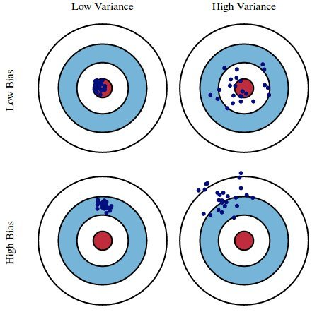
We'd like our models to be in the top left, but in practice that's hard to achieve!
The bias-variance decomposition
- If $H$ is too simple to capture the relationship between $x$s and $y$s in the population, $H$ will underfit to training sets and have high bias.
- If $H$ is overly complex, $H$ will overfit to training sets and have high variance, meaning it will change significantly from one training set to the next.
- Generally:
- Training error reflects bias, not variance.
- Test error reflects both bias and variance.
Navigating the bias-variance tradeoff
- As we collect more data points (i.e. as $n \uparrow$):
- Model variance decreases.
- If $H$ can exactly model the true population relationship between $x$ and $y$ (e.g. cubic), then model bias also decreases.
- If $H$ can't exactly model the true population relationship between $x$ and $y$, then model bias will remain large.
- As we add more features (i.e. as $d \uparrow$):
- Model variance increases, whether or not the feature was useful.
- Adding a useful feature decreases model bias.
- Adding a useless feature doesn't change model bias.
- Example: suppose the actual relationship between $x$ and $y$ in the population is linear, and we fit $H$ using simple linear regression.
- Model bias = 0.
- Model variance $\propto \frac{d}{n}$.
- As $d \uparrow$, model variance $\uparrow$.
- As $n \uparrow$, model variance $\downarrow$.
Read more here.
Question 🤔 (Answer at dsc80.com/q)
Code: fa23q94
(Fa23 Final 9.4)
Determine how each change below affects model bias and variance compared to this model:

For each change, choose all of the following that apply: increase bias, decrease bias, increase variance, decrease variance.
- Add degree 3 polynomial features.
- Add a feature of numbers chosen at random between 0 and 1.
- Collect 100 more points for the training set.
- Don’t use the 'veg' feature.
Train-test splits
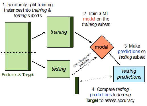
Avoiding overfitting
- We won't know whether our model has overfit to our sample (training data) unless we get to see how well it performs on a new sample from the same population.
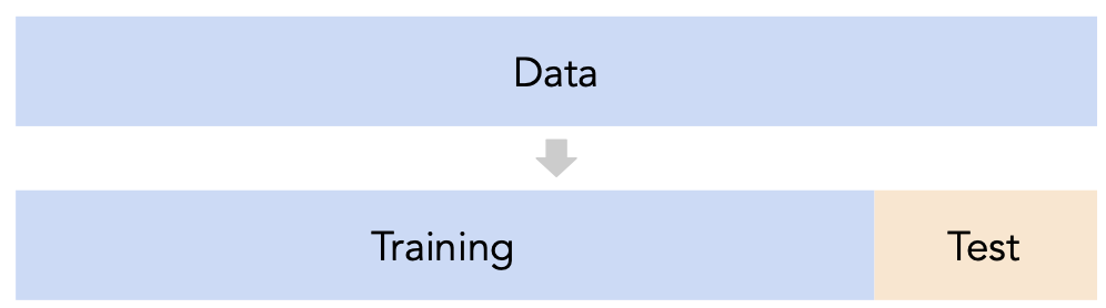
- 💡Idea: Split our sample into a training set and test set.
- Use only the training set to fit the model (i.e. find $w^*$).
- Use the test set to evaluate the model's error (RMSE, $R^2$).
- The test set is like a new sample of data from the same population as the training data!
Train-test split 🚆
sklearn.model_selection.train_test_split implements a train-test split for us! 🙏🏼
If X is an array/DataFrame of features and y is an array/Series of responses,
X_train, X_test, y_train, y_test = train_test_split(X, y, test_size=0.25)
randomly splits the features and responses into training and test sets, such that the test set contains 0.25 of the full dataset.
from sklearn.model_selection import train_test_split
# Read the documentation!
train_test_split?
Signature: train_test_split( *arrays, test_size=None, train_size=None, random_state=None, shuffle=True, stratify=None, ) Docstring: Split arrays or matrices into random train and test subsets. Quick utility that wraps input validation, ``next(ShuffleSplit().split(X, y))``, and application to input data into a single call for splitting (and optionally subsampling) data into a one-liner. Read more in the :ref:`User Guide <cross_validation>`. Parameters ---------- *arrays : sequence of indexables with same length / shape[0] Allowed inputs are lists, numpy arrays, scipy-sparse matrices or pandas dataframes. test_size : float or int, default=None If float, should be between 0.0 and 1.0 and represent the proportion of the dataset to include in the test split. If int, represents the absolute number of test samples. If None, the value is set to the complement of the train size. If ``train_size`` is also None, it will be set to 0.25. train_size : float or int, default=None If float, should be between 0.0 and 1.0 and represent the proportion of the dataset to include in the train split. If int, represents the absolute number of train samples. If None, the value is automatically set to the complement of the test size. random_state : int, RandomState instance or None, default=None Controls the shuffling applied to the data before applying the split. Pass an int for reproducible output across multiple function calls. See :term:`Glossary <random_state>`. shuffle : bool, default=True Whether or not to shuffle the data before splitting. If shuffle=False then stratify must be None. stratify : array-like, default=None If not None, data is split in a stratified fashion, using this as the class labels. Read more in the :ref:`User Guide <stratification>`. Returns ------- splitting : list, length=2 * len(arrays) List containing train-test split of inputs. .. versionadded:: 0.16 If the input is sparse, the output will be a ``scipy.sparse.csr_matrix``. Else, output type is the same as the input type. Examples -------- >>> import numpy as np >>> from sklearn.model_selection import train_test_split >>> X, y = np.arange(10).reshape((5, 2)), range(5) >>> X array([[0, 1], [2, 3], [4, 5], [6, 7], [8, 9]]) >>> list(y) [0, 1, 2, 3, 4] >>> X_train, X_test, y_train, y_test = train_test_split( ... X, y, test_size=0.33, random_state=42) ... >>> X_train array([[4, 5], [0, 1], [6, 7]]) >>> y_train [2, 0, 3] >>> X_test array([[2, 3], [8, 9]]) >>> y_test [1, 4] >>> train_test_split(y, shuffle=False) [[0, 1, 2], [3, 4]] File: ~/miniforge3/envs/dsc80/lib/python3.11/site-packages/sklearn/model_selection/_split.py Type: function
Let's perform a train/test split on our tips dataset.
X = tips.drop('tip', axis=1)
y = tips['tip']
X_train, X_test, y_train, y_test = train_test_split(X, y, test_size=0.2) # We don't have to choose 0.25.
Before proceeding, let's check the sizes of X_train and X_test.
print('Rows in X_train:', X_train.shape[0])
display(X_train.head())
print('Rows in X_test:', X_test.shape[0])
display(X_test.head())
Rows in X_train: 195
| total_bill | sex | smoker | day | time | size | |
|---|---|---|---|---|---|---|
| 4 | 24.59 | Female | No | Sun | Dinner | 4 |
| 209 | 12.76 | Female | Yes | Sat | Dinner | 2 |
| 178 | 9.60 | Female | Yes | Sun | Dinner | 2 |
| 230 | 24.01 | Male | Yes | Sat | Dinner | 4 |
| 5 | 25.29 | Male | No | Sun | Dinner | 4 |
Rows in X_test: 49
| total_bill | sex | smoker | day | time | size | |
|---|---|---|---|---|---|---|
| 146 | 18.64 | Female | No | Thur | Lunch | 3 |
| 224 | 13.42 | Male | Yes | Fri | Lunch | 2 |
| 134 | 18.26 | Female | No | Thur | Lunch | 2 |
| 131 | 20.27 | Female | No | Thur | Lunch | 2 |
| 147 | 11.87 | Female | No | Thur | Lunch | 2 |
X_train.shape[0] / tips.shape[0]
0.7991803278688525
Example train-test split
Steps:
- Fit a model on the training set.
- Evaluate the model on the test set.
tips.head()
| total_bill | tip | sex | smoker | day | time | size | |
|---|---|---|---|---|---|---|---|
| 0 | 16.99 | 1.01 | Female | No | Sun | Dinner | 2 |
| 1 | 10.34 | 1.66 | Male | No | Sun | Dinner | 3 |
| 2 | 21.01 | 3.50 | Male | No | Sun | Dinner | 3 |
| 3 | 23.68 | 3.31 | Male | No | Sun | Dinner | 2 |
| 4 | 24.59 | 3.61 | Female | No | Sun | Dinner | 4 |
X = tips[['total_bill', 'size']] # For this example, we'll use just the already-quantitative columns in tips.
y = tips['tip']
X_train, X_test, y_train, y_test = train_test_split(X, y, test_size=0.2, random_state=1) # random_state is like np.random.seed.
Here, we'll use a stand-alone LinearRegression model without a Pipeline, but this process would work the same if we were using a Pipeline.
lr = LinearRegression()
lr.fit(X_train, y_train)
LinearRegression()In a Jupyter environment, please rerun this cell to show the HTML representation or trust the notebook.
On GitHub, the HTML representation is unable to render, please try loading this page with nbviewer.org.
LinearRegression()
Let's check our model's performance on the training set first.
pred_train = lr.predict(X_train)
rmse_train = root_mean_squared_error(y_train, pred_train)
rmse_train
np.float64(0.9803205287924736)
And the test set:
pred_test = lr.predict(X_test)
rmse_test = root_mean_squared_error(y_test, pred_test)
rmse_test
np.float64(1.1381771291131253)
Since rmse_train and rmse_test are similar, it doesn't seem like our model is overfitting to the training data. If rmse_test was much larger than rmse_train, it would be evidence that our model is unable to generalize well.
Hyperparameters
Example: Polynomial regression
We recently looked at an example of polynomial regression.
fig = util.train_and_plot(train_sample=sample_1, test_sample=sample_2, degs=[1, 3, 25], data_name='Sample 2')
fig.update_layout(title='Trained on Sample 1, Performance on Sample 2')
When building these models:
- We got to choose the degree of the polynomials (i.e. we chose 1, 3, and 25).
- We didn't get to choose the exact formulas for the three polynomials – their formulas were learned from data.
Parameters vs. hyperparameters
A parameter defines the relationship between variables in a model.
- We learn parameters from data.
- For instance, suppose we fit a degree 3 polynomial to data, and end up with
$$H(x) = 1 - 2x + 13x^2 - 4x^3$$
- 1, -2, 13, and -4 are parameters.
- A hyperparameter is a parameter that we get to choose before our model is fit to the data.
- Think of hyperparameters as knobs 🎛 – we get to pick and tune them!
- Polynomial degree was a hyperparameter in the previous example, and we tried three different values: 1, 3, and 25.
- Question: How do we choose the "right" hyperparameter(s)?
Training error vs. test error
- We know that a model's performance on a test set is a good estimate of its ability to generalize to unseen data.
- We want to find the hyperparameter that leads to the best test set performance.
- Idea:
- Come up with a list of hyperparameters to try.
- For each hyperparameter, train the model on the training set and compute its performance on the test set.
- Pick the hyperparameter with the best performance on the test set.
Training error vs. test error
Let's try this strategy on Sample 1 from our earlier example.
We'll try to fit a polynomial model on the dataset; we'll choose the polynomial's degree from the list [1, 2, ..., 25].
px.scatter(sample_1, x='x', y='y', title='Sample 1')
First, we perform a train-test split.
X = sample_1[['x']]
y = sample_1['y']
X_train, X_test, y_train, y_test = train_test_split(X, y, random_state=100)
Polynomial degree vs. train/test error
Now, we'll create models with degree-1 through degree-25 polynomial features and compute their train and test errors.
train_errs = []
test_errs = []
for d in range(1, 26):
pl = make_pipeline(PolynomialFeatures(d), LinearRegression())
pl.fit(X_train, y_train)
train_errs.append(root_mean_squared_error(y_train, pl.predict(X_train)))
test_errs.append(root_mean_squared_error(y_test, pl.predict(X_test)))
errs = pd.DataFrame({'Train Error': train_errs, 'Test Error': test_errs})
Let's look at the plots of training error vs. degree and test error vs. degree.
fig = px.line(errs)
fig.update_layout(showlegend=True, xaxis_title='Polynomial Degree', yaxis_title='RMSE')
- Training error appears to decrease as polynomial degree increases.
- Test error appears to decrease until a "valley", and then increases again.
- Here, we'd choose a degree of 3, since that degree has the lowest test error.
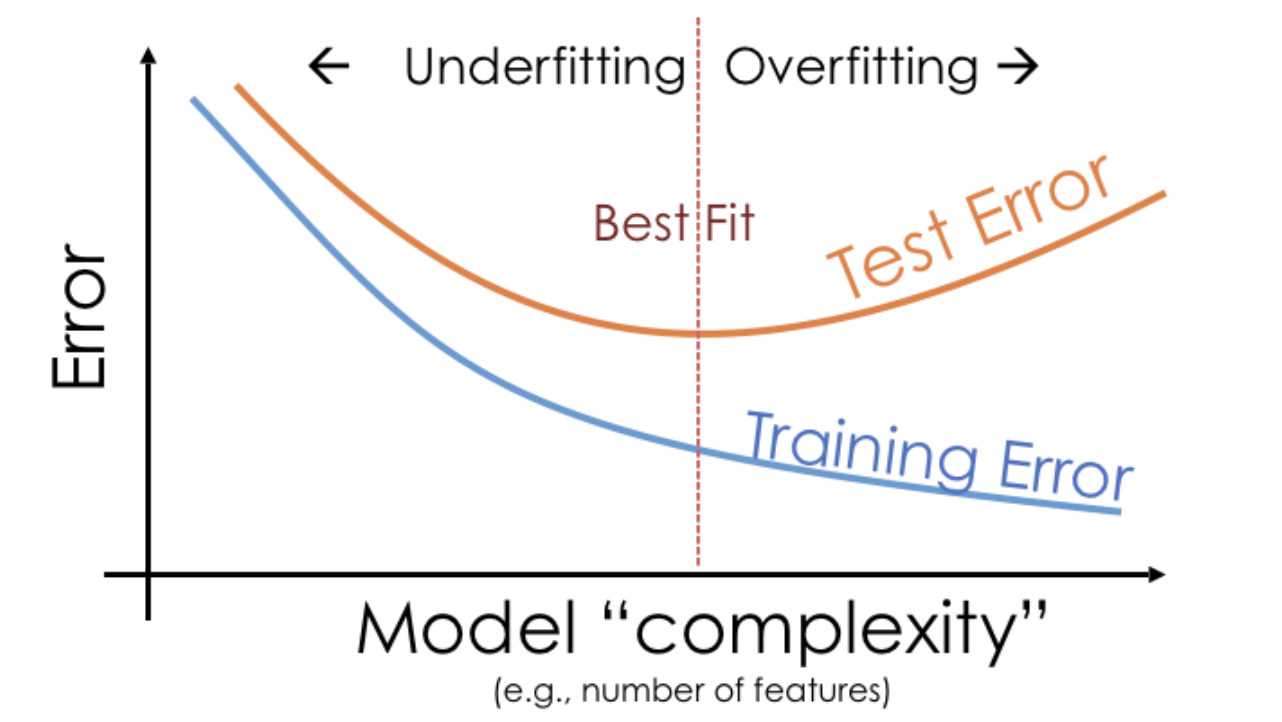
We pick the hyperparameter(s) at the "valley" of test error.
Note that training error tends to underestimate test error, but it doesn't have to – i.e., it is possible for test error to be lower than training error (say, if the test set is "easier" to predict than the training set).
Conducting train-test splits
- Recall, training data is used to fit our model, and test data is used to evaluate our model.
- Question: How should we split?
sklearn'strain_test_splitsplits randomly, which usually works well.- However, if there is some element of time in the training data (say, when predicting the future price of a stock), a better split is "past" and "future".
- Question: How large should the split be, e.g. 90%-10% vs. 75%-25%?
- There's a tradeoff – a larger training set should lead to a "better" model, while a larger test set should lead to a better estimate of our model's ability to generalize.
- There's no "right" choice, but we usually choose between 10% to 25% for the test set.
But wait...
- With our current strategy, we are choosing the hyperparameter that creates the model that performs best on the test set.
- As such, we are overfitting to the test set – the best hyperparameter for the test set might not be the best hyperparameter for a totally unseen dataset!
- It seems like we need another split.
Summary, next time
Summary
- We want to build models that generalize well to unseen data.
- Models that have high bias are too simple to represent complex relationships in data, and underfit.
- Models that have high variance are overly complex for the relationships in the data, and vary a lot when fit on different datasets. Such models overfit to the training data.
- A model's training error tends to decrease as model complexity increases, while its test error tends to decrease, before reaching a "sweet spot" and increasing again.
- A hyperparameter is a configuration that we choose before training a model; an important task in machine learning is selecting "good" hyperparameters.
Next time
We can't choose model hyperparameters just by using a train-test split, because this strategy overfits to the test data.
Is there a better way to choose model hyperparameters? Yes: cross-validation.