from dsc80_utils import *
import lec16_util as util
Agenda 📆
- Hyperparameters.
- Cross-validation.
- Decision trees.
Review: Pipelines
from sklearn.pipeline import make_pipeline
from sklearn.preprocessing import FunctionTransformer, OneHotEncoder, Binarizer
from sklearn.compose import make_column_transformer
from sklearn.linear_model import LinearRegression
tips = px.data.tips()
def is_weekend(s):
# The input to is_weekend is a Series!
return s.replace({'Thur': 'Weekday', 'Fri': 'Weekday'})
pl_day = make_pipeline(
FunctionTransformer(is_weekend),
OneHotEncoder(),
)
col_trans = make_column_transformer(
(pl_day, ['day']),
(OneHotEncoder(drop='first'), ['sex', 'smoker', 'time']),
(Binarizer(threshold=2), ['size']),
remainder='passthrough',
force_int_remainder_cols=False,
)
pl = make_pipeline(
col_trans,
LinearRegression(),
)
pl.fit(tips.drop('tip', axis=1), tips['tip'])
Pipeline(steps=[('columntransformer',
ColumnTransformer(force_int_remainder_cols=False,
remainder='passthrough',
transformers=[('pipeline',
Pipeline(steps=[('functiontransformer',
FunctionTransformer(func=<function is_weekend at 0x16f8ace00>)),
('onehotencoder',
OneHotEncoder())]),
['day']),
('onehotencoder',
OneHotEncoder(drop='first'),
['sex', 'smoker', 'time']),
('binarizer',
Binarizer(threshold=2),
['size'])])),
('linearregression', LinearRegression())])In a Jupyter environment, please rerun this cell to show the HTML representation or trust the notebook. On GitHub, the HTML representation is unable to render, please try loading this page with nbviewer.org.
Pipeline(steps=[('columntransformer',
ColumnTransformer(force_int_remainder_cols=False,
remainder='passthrough',
transformers=[('pipeline',
Pipeline(steps=[('functiontransformer',
FunctionTransformer(func=<function is_weekend at 0x16f8ace00>)),
('onehotencoder',
OneHotEncoder())]),
['day']),
('onehotencoder',
OneHotEncoder(drop='first'),
['sex', 'smoker', 'time']),
('binarizer',
Binarizer(threshold=2),
['size'])])),
('linearregression', LinearRegression())])ColumnTransformer(force_int_remainder_cols=False, remainder='passthrough',
transformers=[('pipeline',
Pipeline(steps=[('functiontransformer',
FunctionTransformer(func=<function is_weekend at 0x16f8ace00>)),
('onehotencoder',
OneHotEncoder())]),
['day']),
('onehotencoder', OneHotEncoder(drop='first'),
['sex', 'smoker', 'time']),
('binarizer', Binarizer(threshold=2),
['size'])])['day']
FunctionTransformer(func=<function is_weekend at 0x16f8ace00>)
OneHotEncoder()
['sex', 'smoker', 'time']
OneHotEncoder(drop='first')
['size']
Binarizer(threshold=2)
['total_bill']
passthrough
LinearRegression()
Review: Hyperparameters
np.random.seed(23) # For reproducibility.
def sample_from_pop(n=100):
x = np.linspace(-2, 3, n)
y = x ** 3 + (np.random.normal(0, 3, size=n))
return pd.DataFrame({'x': x, 'y': y})
sample_1 = sample_from_pop()
sample_2 = sample_from_pop()
px.scatter(sample_1, x='x', y='y', title='Sample 1')
Example: Polynomial regression
We recently looked at an example of polynomial regression.
fig = util.train_and_plot(train_sample=sample_1, test_sample=sample_2, degs=[1, 3, 25], data_name='Sample 2')
fig.update_layout(title='Trained on Sample 1, Performance on Sample 2')
When building these models:
- We got to choose the degree of the polynomials (i.e. we chose 1, 3, and 25).
- We didn't get to choose the exact formulas for the three polynomials – their formulas were learned from data.
Parameters vs. hyperparameters
A parameter defines the relationship between variables in a model.
- We learn parameters from data.
- For instance, suppose we fit a degree 3 polynomial to data, and end up with
$$H(x) = 1 - 2x + 13x^2 - 4x^3$$
- 1, -2, 13, and -4 are parameters.
- A hyperparameter is a parameter that we get to choose before our model is fit to the data.
- Think of hyperparameters as knobs 🎛 – we get to pick and tune them!
- Polynomial degree was a hyperparameter in the previous example, and we tried three different values: 1, 3, and 25.
- Question: How do we choose the "right" hyperparameter(s)?
Training error vs. test error
- We know that a model's performance on a test set is a good estimate of its ability to generalize to unseen data.
- We want to find the hyperparameter that leads to the best test set performance.
- Idea:
- Come up with a list of hyperparameters to try.
- For each hyperparameter, train the model on the training set and compute its performance on the test set.
- Pick the hyperparameter with the best performance on the test set.
Training error vs. test error
Let's try this strategy on Sample 1 from our earlier example.
We'll try to fit a polynomial model on the dataset; we'll choose the polynomial's degree from the list [1, 2, ..., 25].
px.scatter(sample_1, x='x', y='y', title='Sample 1')
First, we perform a train-test split.
from sklearn.model_selection import train_test_split
X = sample_1[['x']]
y = sample_1['y']
X_train, X_test, y_train, y_test = train_test_split(X, y, random_state=100)
Polynomial degree vs. train/test error
Now, we'll create models with degree-1 through degree-25 polynomial features and compute their train and test errors.
from sklearn.metrics import root_mean_squared_error
from sklearn.preprocessing import PolynomialFeatures
train_errs = []
test_errs = []
for d in range(1, 26):
pl = make_pipeline(PolynomialFeatures(d), LinearRegression())
pl.fit(X_train, y_train)
train_errs.append(root_mean_squared_error(y_train, pl.predict(X_train)))
test_errs.append(root_mean_squared_error(y_test, pl.predict(X_test)))
errs = pd.DataFrame({'Train Error': train_errs, 'Test Error': test_errs})
Let's look at the plots of training error vs. degree and test error vs. degree.
fig = px.line(errs)
fig.update_layout(showlegend=True, xaxis_title='Polynomial Degree', yaxis_title='RMSE')
- Training error appears to decrease as polynomial degree increases.
- Test error appears to decrease until a "valley", and then increases again.
- Here, we'd choose a degree of 3, since that degree has the lowest test error.

We pick the hyperparameter(s) at the "valley" of test error.
Note that training error tends to underestimate test error, but it doesn't have to – i.e., it is possible for test error to be lower than training error (say, if the test set is "easier" to predict than the training set).
Conducting train-test splits
- Recall, training data is used to fit our model, and test data is used to evaluate our model.
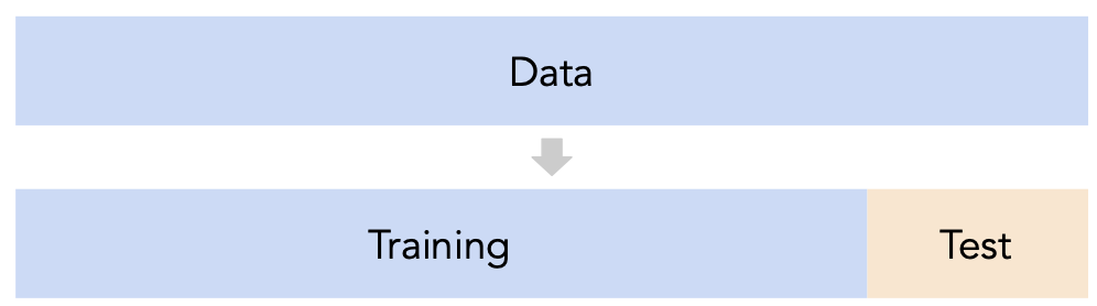
- Question: How should we split?
sklearn'strain_test_splitsplits randomly, which usually works well.- However, if there is some element of time in the training data (say, when predicting the future price of a stock), a better split is "past" and "future".
- Question: How large should the split be, e.g. 90%-10% vs. 75%-25%?
- There's a tradeoff – a larger training set should lead to a "better" model, while a larger test set should lead to a better estimate of our model's ability to generalize.
- There's no "right" choice, but we usually choose between 10% to 25% for the test set.
But wait...
- With our current strategy, we are choosing the hyperparameter that creates the model that performs best on the test set.
- As such, we are overfitting to the test set – the best hyperparameter for the test set might not be the best hyperparameter for a totally unseen dataset!
- It seems like we need another split.
Cross-validation
Idea: A single validation set
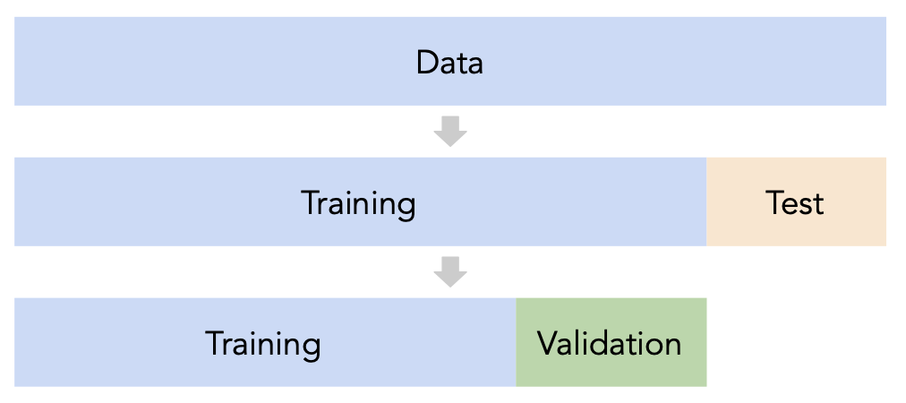
- Split the data into three sets: training, validation, and test.
- For each hyperparameter choice, train the model only on the training set, and evaluate the model's performance on the validation set.
- Find the hyperparameter with the best validation performance.
- Retrain the final model on the training and validation sets, and report its performance on the test set.
Issue: This strategy is too dependent on the validation set, which may be small and/or not a representative sample of the data. We're not going to do this. ❌
A better idea: $k$-fold cross-validation
Instead of relying on a single validation set, we can create $k$ validation sets, where $k$ is some positive integer (5 in the example below).
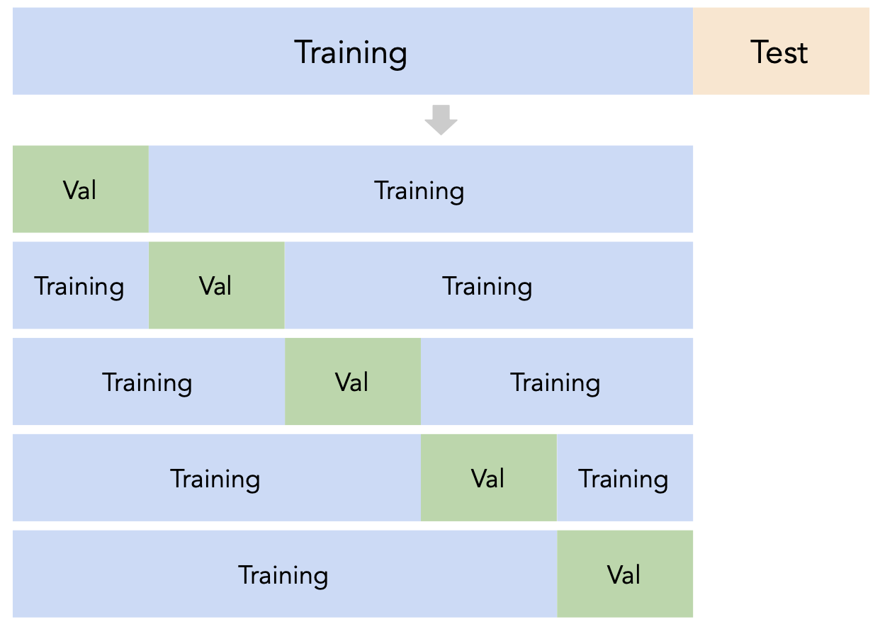
Since each data point is used for training $k-1$ times and validation once, the (averaged) validation performance should be a good metric of a model's ability to generalize to unseen data.
$k$-fold cross-validation (or simply "cross-validation") is the technique we will use for finding hyperparameters, or more generally, for choosing between different possible models. It's what you should use in your Final Project! ✅
Creating folds in sklearn
sklearn has a KFold class that splits data into training and validation folds.
from sklearn.model_selection import KFold
Let's use a simple dataset for illustration.
data = np.arange(10, 70, 10)
data
array([10, 20, 30, 40, 50, 60])
Let's instantiate a KFold object with $k=3$.
kfold = KFold(3, shuffle=False)
kfold
KFold(n_splits=3, random_state=None, shuffle=False)
Finally, let's use kfold to split data:
for train, val in kfold.split(data):
print(f'train: {data[train]}, validation: {data[val]}')
train: [30 40 50 60], validation: [10 20] train: [10 20 50 60], validation: [30 40] train: [10 20 30 40], validation: [50 60]
Note that each value in data is used for validation exactly once and for training exactly twice. Also note that because we set shuffle=True the folds are not simply [10, 20], [30, 40], and [50, 60].
$k$-fold cross-validation
First, shuffle the entire training set randomly and split it into $k$ disjoint folds, or "slices". Then:
- For each hyperparameter:
- For each slice:
- Let the slice be the "validation set", $V$.
- Let the rest of the data be the "training set", $T$.
- Train a model using the selected hyperparameter on the training set $T$.
- Evaluate the model on the validation set $V$.
- Compute the average validation score (e.g. RMSE) for the particular hyperparameter.
- For each slice:
- Choose the hyperparameter with the best average validation score.
$k$-fold cross-validation in sklearn
While you could manually use KFold to perform cross-validation, the cross_val_score function in sklearn implements $k$-fold cross-validation for us!
cross_val_score(estimator, X_train, y_train, cv)
Specifically, it takes in:
- A
Pipelineor estimator that has not already beenfit. - Training data.
- A value of $k$ (through the
cvargument). - (Optionally) A
scoringmetric.
and performs $k$-fold cross-validation, returning the values of the scoring metric on each fold.
from sklearn.model_selection import cross_val_score
$k$-fold cross-validation in sklearn
- Let's perform $k$-fold cross validation in order to help us pick a degree for polynomial regression from the list [1, 2, ..., 25].
- We'll use $k=5$ since it's a common choice (and the default in
sklearn).
- For the sake of this example, we'll suppose
sample_1is our "training + validation data", i.e. that our test data is in some other dataset.- If this were not true, we'd first need to split
sample_1into separate training and test sets.
- If this were not true, we'd first need to split
errs_df = pd.DataFrame()
for d in range(1, 26):
pl = make_pipeline(PolynomialFeatures(d), LinearRegression())
# The `scoring` argument is used to specify that we want to compute the RMSE;
# the default is R^2. It's called "neg" RMSE because,
# by default, sklearn likes to "maximize" scores, and maximizing -RMSE is the same
# as minimizing RMSE.
errs = cross_val_score(pl, sample_1[['x']], sample_1['y'],
cv=KFold(5, shuffle=True), scoring='neg_root_mean_squared_error')
errs_df[f'Deg {d}'] = -errs # Negate to turn positive (sklearn computed negative RMSE).
errs_df.index = [f'Fold {i}' for i in range(1, 6)]
errs_df.index.name = 'Validation Fold'
Next class, we'll look at how to implement this procedure without needing to for-loop over values of d.
$k$-fold cross-validation in sklearn
Note that for each choice of degree (our hyperparameter), we have five RMSEs, one for each "fold" of the data. This means that in total, $5 \cdot 25 = 125$ models were trained/fit to data!
errs_df
| Deg 1 | Deg 2 | Deg 3 | Deg 4 | ... | Deg 22 | Deg 23 | Deg 24 | Deg 25 | |
|---|---|---|---|---|---|---|---|---|---|
| Validation Fold | |||||||||
| Fold 1 | 4.79 | 12.81 | 5.04 | 4.93 | ... | 8.77e+06 | 6.57e+07 | 1.41e+08 | 5.90e+08 |
| Fold 2 | 3.97 | 5.36 | 3.19 | 3.22 | ... | 2.93e+01 | 7.85e+01 | 7.53e+01 | 3.13e+01 |
| Fold 3 | 4.77 | 2.56 | 2.08 | 2.11 | ... | 3.03e+01 | 3.09e+01 | 4.24e+01 | 3.72e+01 |
| Fold 4 | 6.13 | 4.66 | 2.93 | 2.93 | ... | 6.27e+00 | 3.33e+01 | 5.80e+01 | 9.69e+00 |
| Fold 5 | 11.70 | 11.92 | 3.24 | 4.37 | ... | 8.36e+06 | 2.28e+08 | 8.17e+08 | 6.63e+09 |
5 rows × 25 columns
We should choose the degree with the lowest average validation RMSE.
errs_df.mean().idxmin()
'Deg 3'
Note that if we didn't perform $k$-fold cross-validation, but instead just used a single validation set, we may have ended up with a different result:
errs_df.idxmin(axis=1)
Validation Fold Fold 1 Deg 1 Fold 2 Deg 6 Fold 3 Deg 8 Fold 4 Deg 3 Fold 5 Deg 3 dtype: object
Question 🤔 (Answer at dsc80.com/q)
Code: folds
The RMSEs in Folds 1 and 5 are much higher than in other folds. Why? How we might fix this?
px.scatter(sample_1, x='x', y='y', title='Sample 1')
Another example: Tips
We can also use $k$-fold cross-validation to determine which subset of features to use in a linear model that predicts tips by making one pipeline for each subset of features we want to evaluate.
# make_column_transformer is a shortcut for the ColumnTransformer class
from sklearn.compose import make_column_transformer, make_column_selector
from sklearn.preprocessing import FunctionTransformer, OneHotEncoder
As we should always do, we'll perform a train-test split on tips and will only use the training data for cross-validation.
tips = sns.load_dataset('tips')
tips.head()
| total_bill | tip | sex | smoker | day | time | size | |
|---|---|---|---|---|---|---|---|
| 0 | 16.99 | 1.01 | Female | No | Sun | Dinner | 2 |
| 1 | 10.34 | 1.66 | Male | No | Sun | Dinner | 3 |
| 2 | 21.01 | 3.50 | Male | No | Sun | Dinner | 3 |
| 3 | 23.68 | 3.31 | Male | No | Sun | Dinner | 2 |
| 4 | 24.59 | 3.61 | Female | No | Sun | Dinner | 4 |
X = tips.drop('tip', axis=1)
y = tips['tip']
X_train, X_test, y_train, y_test = train_test_split(X, y, test_size=0.2, random_state=1)
# A dictionary that maps names to Pipeline objects.
select = FunctionTransformer(lambda x: x)
pipes = {
'total_bill only': make_pipeline(
make_column_transformer( (select, ['total_bill']) ),
LinearRegression(),
),
'total_bill + size': make_pipeline(
make_column_transformer( (select, ['total_bill', 'size']) ),
LinearRegression(),
),
'total_bill + size + OHE smoker': make_pipeline(
make_column_transformer(
(select, ['total_bill', 'size']),
(OneHotEncoder(drop='first'), ['smoker']),
),
LinearRegression(),
),
'total_bill + size + OHE all': make_pipeline(
make_column_transformer(
(select, ['total_bill', 'size']),
(OneHotEncoder(drop='first'), ['smoker', 'sex', 'time', 'day']),
),
LinearRegression(),
),
}
pipe_df = pd.DataFrame()
for pipe in pipes:
errs = cross_val_score(pipes[pipe], X_train, y_train,
cv=5, scoring='neg_root_mean_squared_error')
pipe_df[pipe] = -errs
pipe_df.index = [f'Fold {i}' for i in range(1, 6)]
pipe_df.index.name = 'Validation Fold'
pipe_df
| total_bill only | total_bill + size | total_bill + size + OHE smoker | total_bill + size + OHE all | |
|---|---|---|---|---|
| Validation Fold | ||||
| Fold 1 | 1.32 | 1.27 | 1.27 | 1.29 |
| Fold 2 | 0.95 | 0.92 | 0.93 | 0.93 |
| Fold 3 | 0.77 | 0.86 | 0.86 | 0.87 |
| Fold 4 | 0.85 | 0.84 | 0.84 | 0.86 |
| Fold 5 | 1.10 | 1.07 | 1.07 | 1.08 |
pipe_df.mean()
total_bill only 1.00 total_bill + size 0.99 total_bill + size + OHE smoker 0.99 total_bill + size + OHE all 1.01 dtype: float64
pipe_df.mean().idxmin()
'total_bill + size + OHE smoker'
Even though the third model has the lowest average validation RMSE, its average validation RMSE is very close to that of the other, simpler models, and as a result we'd likely use the simplest model in practice.
Question 🤔 (Answer at dsc80.com/q)
Code: 10cv
- Suppose you have a training dataset with 1000 rows.
- You want to decide between 20 hyperparameters for a particular model.
- To do so, you perform 10-fold cross-validation.
- How many times is the first row in the training dataset (
X.iloc[0]) used for training a model?
Summary: Generalization
- Split the data into two sets: training and test.
- Use only the training data when designing, training, and tuning the model.
- Use $k$-fold cross-validation to choose hyperparameters and estimate the model's ability to generalize.
- Do not ❌ look at the test data in this step!
- Commit to your final model and train it using the entire training set.
- Test the data using the test data. If the performance (e.g. RMSE) is not acceptable, return to step 2.
- Finally, train on all available data and ship the model to production! 🛳
🚨 This is the process you should always use! 🚨
Decision trees 🌲

Decision trees can be used for both regression and classification. We'll start by using them for classification.
Example: Should I get groceries?
Decision trees make classifications by answering a series of yes/no questions.
Should I go to Trader Joe's to buy groceries today?

Internal nodes of trees involve questions; leaf nodes make predictions $H(x)$.

Example: Predicting diabetes
diabetes = pd.read_csv(Path('data') / 'diabetes.csv')
display_df(diabetes, cols=9)
| Pregnancies | Glucose | BloodPressure | SkinThickness | Insulin | BMI | DiabetesPedigreeFunction | Age | Outcome | |
|---|---|---|---|---|---|---|---|---|---|
| 0 | 6 | 148 | 72 | 35 | 0 | 33.6 | 0.63 | 50 | 1 |
| 1 | 1 | 85 | 66 | 29 | 0 | 26.6 | 0.35 | 31 | 0 |
| 2 | 8 | 183 | 64 | 0 | 0 | 23.3 | 0.67 | 32 | 1 |
| ... | ... | ... | ... | ... | ... | ... | ... | ... | ... |
| 765 | 5 | 121 | 72 | 23 | 112 | 26.2 | 0.24 | 30 | 0 |
| 766 | 1 | 126 | 60 | 0 | 0 | 30.1 | 0.35 | 47 | 1 |
| 767 | 1 | 93 | 70 | 31 | 0 | 30.4 | 0.32 | 23 | 0 |
768 rows × 9 columns
# 0 means no diabetes, 1 means yes diabetes.
diabetes['Outcome'].value_counts()
'Glucose'is measured in mg/dL (milligrams per deciliter).
'BMI'is calculated as $\text{BMI} = \frac{\text{weight (kg)}}{\left[ \text{height (m)} \right]^2}$.
- Let's use
'Glucose'and'BMI'to predict whether or not a patient has diabetes ('Outcome').
Exploring the dataset
First, a train-test split:
from sklearn.model_selection import train_test_split
X_train, X_test, y_train, y_test = (
train_test_split(diabetes[['Glucose', 'BMI']], diabetes['Outcome'], random_state=1)
)
Class 0 (orange) is "no diabetes" and class 1 (blue) is "diabetes".
fig = (
X_train.assign(Outcome=y_train.astype(str))
.plot(kind='scatter', x='Glucose', y='BMI', color='Outcome',
color_discrete_map={'0': 'orange', '1': 'blue'},
title='Relationship between Glucose, BMI, and Diabetes')
)
fig
Building a decision tree
Let's build a decision tree and interpret the results.
The relevant class is DecisionTreeClassifier, from sklearn.tree.
from sklearn.tree import DecisionTreeClassifier
Note that we fit it the same way we fit earlier estimators.
You may wonder what max_depth and criterion do – more on this soon!
dt = DecisionTreeClassifier(max_depth=2, criterion='entropy')
dt.fit(X_train, y_train)
DecisionTreeClassifier(criterion='entropy', max_depth=2)In a Jupyter environment, please rerun this cell to show the HTML representation or trust the notebook.
On GitHub, the HTML representation is unable to render, please try loading this page with nbviewer.org.
DecisionTreeClassifier(criterion='entropy', max_depth=2)
Visualizing decision trees
Our fit decision tree is like a "flowchart", made up of a series of questions.
As before, orange is "no diabetes" and blue is "diabetes".
from sklearn.tree import plot_tree
plt.figure(figsize=(15, 5))
plot_tree(dt, feature_names=X_train.columns, class_names=['no db', 'yes db'],
filled=True, fontsize=15, impurity=False);

- To classify a new data point, we start at the top and answer the first question (i.e. "Glucose <= 129.5").
- If the answer is "Yes", we move to the left branch, otherwise we move to the right branch.
- We repeat this process until we end up at a leaf node, at which point we predict the most common class in that node.
- Note that each node has a
valueattribute, which describes the number of training individuals of each class that fell in that node.
- Note that each node has a
# Note that the left node at depth 2 has a `value` of [304, 78].
y_train[X_train.query('Glucose <= 129.5').index].value_counts()
Evaluating classifiers
The most common evaluation metric in classification is accuracy:
$$\text{accuracy} = \frac{\text{\# data points classified correctly}}{\text{\# data points}}$$
(dt.predict(X_train) == y_train).mean()
np.float64(0.765625)
The score method of a classifier computes accuracy by default (just like the score method of a regressor computes $R^2$ by default). We want our classifiers to have high accuracy.
# Training accuracy – same number as above
dt.score(X_train, y_train)
0.765625
# Testing accuracy
dt.score(X_test, y_test)
0.7760416666666666
Reflection
- Decision trees are easily interpretable: it is clear how they make their predictions.
- They work with categorical data without needing to use one hot encoding.
- They also can be used in multi-class classification problems, e.g. when there are more than 2 possible outcomes.
- The decision boundary of a decision tree can be arbitrarily complicated.
- How are decision trees trained?
How are decision trees trained?
Pseudocode:
def make_tree(X, y):
if all points in y have the same label C:
return Leaf(C)
f = best splitting feature # e.g. Glucose or BMI
v = best splitting value # e.g. 129.5
X_left, y_left = X, y where (X[f] <= v)
X_right, y_right = X, y where (X[f] > v)
left = make_tree(X_left, y_left)
right = make_tree(X_right, y_right)
return Node(f, v, left, right)
make_tree(X_train, y_train)
How do we measure the quality of a split?
Our pseudocode for training a decision tree relies on finding the best way to "split" a node – that is, the best question to ask to help us narrow down which class to predict.
Intuition: Suppose the distribution within a node looks like this (colors represent classes):
Split A:
- "Yes": 🟠🟠🟠🔵🔵🔵
- "No": 🟠🟠🟠🔵🔵🔵🔵
Split B:
- "Yes": 🔵🔵🔵🔵🔵🔵
- "No": 🔵🟠🟠🟠🟠🟠🟠
Which split is "better"?
Split B, because there is "less uncertainty" in the resulting nodes in Split B than there is in Split A. Let's try and quantify this!
Entropy
- For each class $C$ within a node, define $p_C$ as the proportion of points with that class.
- For example, the two classes may be "yes diabetes" and "no diabetes".
- The surprise of drawing a point from the node at random and having it be class $C$ is:
$$ \log_2 \left(\frac{1}{p_C}\right) = - \log_2 p_C $$
- The entropy of a node is the average surprise over all classes:
\begin{align} \text{entropy} &= - \sum_C p_C \log_2 p_C \end{align}
- The entropy of 🟠🟠🟠🟠🟠🟠🟠🟠 is $ -1 \log_2(1) = 0 $.
- The entropy of 🟠🟠🟠🟠🔵🔵🔵🔵 is $ -0.5 \log_2(0.5) - 0.5 \log_2(0.5) = 1$.
- The entropy of 🟠🔵🟢🟡🟣 is $ - \log_2 \frac{1}{5} = \log_2(5) $
- In general, if a node has $n$ points, all with different labels, the entropy of the node is $ \log_2(n) $.
Example entropy calculation
Suppose we have:
Split A:
- "Yes": 🟠🟠🟠🟠🟠🟠🔵
- "No": 🟠🟠🟠🟠🟠🟠🔵🔵🔵🔵🔵
Split B:
- "Yes": 🟠🟠🟠🟠🟠🟠🔵🔵🔵
- "No": 🟠🟠🟠🟠🟠🟠🔵🔵🔵
We choose the split that has the lowest weighted entropy, that is:
$$\text{entropy of split} = \frac{\# \text{Yes}}{\# \text{Yes} + \# \text{No}} \cdot \text{entropy(Yes)} + \frac{\# \text{No}}{\# \text{Yes} + \# \text{No}} \cdot \text{entropy(No)}$$
def entropy(node):
props = pd.Series(list(node)).value_counts(normalize=True)
return -sum(props * np.log2(props))
def weighted_entropy(yes_node, no_node):
yes_entropy = entropy(yes_node)
no_entropy = entropy(no_node)
yes_weight = len(yes_node) / (len(yes_node) + len(no_node))
return yes_weight * yes_entropy + (1 - yes_weight) * no_entropy
# Split A:
weighted_entropy("🟠🟠🟠🟠🟠🟠🔵", "🟠🟠🟠🟠🟠🟠🔵🔵🔵🔵🔵")
# Split B:
weighted_entropy("🟠🟠🟠🟠🟠🟠🔵🔵🔵", "🟠🟠🟠🟠🟠🟠🔵🔵🔵")
Split A has the lower weighted entropy, so we'll use it.
Understanding entropy
plt.figure(figsize=(15, 5))
plot_tree(dt, feature_names=X_train.columns, class_names=['no db', 'yes db'],
filled=True, fontsize=15, impurity=True);

We can recreate the entropy calculations above! Note that the default DecisionTreeClassifier uncertaintly metric isn't entropy; it used entropy because we set criterion='entropy' when defining dt. (The default metric, Gini impurity, is perfectly fine too!)
# The first node at depth 2 has an entropy of 0.73,
# both told to us above and verified here!
entropy([0] * 304 + [1] * 78)
Tree depth
Decision trees are trained by recursively picking the best split until:
- all "leaf nodes" only contain training examples from a single class (good), or
- it is impossible to split leaf nodes any further (not good).
By default, there is no "maximum depth" for a decision tree. As such, without restriction, decision trees tend to be very deep.
dt_no_max = DecisionTreeClassifier()
dt_no_max.fit(X_train, y_train)
DecisionTreeClassifier()In a Jupyter environment, please rerun this cell to show the HTML representation or trust the notebook.
On GitHub, the HTML representation is unable to render, please try loading this page with nbviewer.org.
DecisionTreeClassifier()
A decision tree fit on our training data has a depth of around 20! (It is so deep that tree.plot_tree errors when trying to plot it.)
dt_no_max.tree_.max_depth
22
At first, this tree seems "better" than our tree of depth 2, since its training accuracy is much much higher:
dt_no_max.score(X_train, y_train)
0.9913194444444444
# Depth 2 tree.
dt.score(X_train, y_train)
0.765625
But recall, we truly care about test set performance, and this decision tree has worse accuracy on the test set than our depth 2 tree.
dt_no_max.score(X_test, y_test)
0.71875
# Depth 2 tree.
dt.score(X_test, y_test)
0.7760416666666666
Decision trees and overfitting
- Decision trees have a tendency to overfit. Why is that?
- Unlike linear classification techniques (like logistic regression or SVMs), decision trees are non-linear.
- They are also "non-parametric" – there are no $w^*$s to learn.
- While being trained, decision trees ask enough questions to effectively memorize the correct response values in the training set. However, the relationships they learn are often overfit to the noise in the training set, and don't generalize well.
fig
- A decision tree whose depth is not restricted will achieve 100% accuracy on any training set, as long as there are no "overlapping values" in the training set.
- Two values overlap when they have the same features $x$ but different response values $y$ (e.g. if two patients have the same glucose levels and BMI, but one has diabetes and one doesn't).
- One solution: Make the decision tree "less complex" by limiting the maximum depth.
Since sklearn.tree's plot_tree can't visualize extremely large decision trees, let's create and visualize some smaller decision trees.
trees = {}
for d in [2, 4, 8]:
trees[d] = DecisionTreeClassifier(max_depth=d, random_state=1)
trees[d].fit(X_train, y_train)
plt.figure(figsize=(15, 5), dpi=100)
plot_tree(trees[d], feature_names=X_train.columns, class_names=['no db', 'yes db'],
filled=True, rounded=True, impurity=False)
plt.show()


As tree depth increases, complexity increases, and our trees are more prone to overfitting. This means model bias decreases, but model variance increases.
Question: What is the "right" maximum depth to choose?
Hyperparameters for decision trees
max_depthis a hyperparameter forDecisionTreeClassifier.
- There are many more hyperparameters we can tweak; look at the documentation for examples.
min_samples_split: The minimum number of samples required to split an internal node.criterion: The function to measure the quality of a split ('gini'or'entropy').
- To ensure that our model generalizes well to unseen data, we need an efficient technique for trying different combinations of hyperparameters!
- We'll see that technique next time:
GridSearchCV.
Question 🤔 (Answer at dsc80.com/q)
Code: trees
(Fa23 Final 10.1)
Suppose we fit decision trees of varying depths to predict 'y' using 'x1' and 'x2'. The entire training set is shown in the table below.
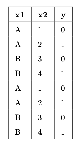
What is:
- The entropy of a node containing all the training points.
- The lowest possible entropy of a node in a fitted tree with depth 1 (two leaf nodes).
- The lowest possible entropy of a node in a fitted tree with depth 2 (four leaf nodes).
Summary, next time
Summary
- A hyperparameter is a configuration that we choose before training a model; an important task in machine learning is selecting "good" hyperparameters.
- To choose hyperparameters, we use $k$-fold cross-validation. This technique is standard, and you are expected to use it in the Final Project!
- See Summary: Generalization for more.
- Decision trees can be used for both regression and classification; we've used them for classification.
- Decision trees are trained recursively. Each node corresponds to a "yes" or "no" question.
- To decide which "yes" or "no" question to ask, we choose the question with the lowest weighted entropy.
Next time
- An efficient technique for trying different combinations of hyperparameters.
- In other words, performing $k$-fold cross-validation without a
for-loop.
- In other words, performing $k$-fold cross-validation without a
- Techniques for evaluating classifiers beyond accuracy.
- You'll need this for the Final Project!